Graduate School
“Stuck. What it is, I think there is a jump some people have to make, sometimes, and if they don’t do it, then they’re stuck good … And Rudy never did it.”
“Like my father wanting to get me out of Maas? Is that a jump?”
“No. Some jumps you have to decide on for yourself. Just figure there’s something better waiting for you somewhere….” He paused, feeling suddenly ridiculous, and bit into the sandwich.
After spending a fair amount of time in industry, I’ve decided its fair time to change directions, to make a jump. This month I’ll be returning to school to work on my master’s degree in Computer Science. Based on what makes me happy, and where I’d like to take my career, it’s the right path and the right time to make this change. I’m looking forward to making the most of it.
As far as what it means for the site, it’s tough to say. August 8th was the six year anniversary of the site and after writing and publishing my interests for so long, it makes sense to continue to do so, but on the same hand, time is precious. So we’ll see. As always, take a look through the archive, follow by email, or by RSS for the latest happenings.
3D Printed Toy Robot
 |
Introduction
At the beginning of the year I decided to change my approach to working on personal projects; in short, more time on quality and less on quantity. With that mindset I thought about my interests and how they could come together to form an interdisciplinary project that would be ambitious, but doable. After much thought, I zeroed in on mechatronics -the interplay of form, computation, electronics and mechanics- and began to explore how I could draw from these disciplines to form the foundation of my next project.
Like most people coming from a software background, much of what I work on is abstract in nature. Every once in a while I have a strong desire to work on something tangible. Lacking the proper space and tools to work with traditional mediums like wood and metal, I thought about newer mediums I’d read about and directed my attention to 3D printing. Despite being 30 years old, the technology has only become accessible to consumers within the past seven years with the launch of several online services and open source printers. Having watched this growth, I was curious about the technology and decided it would be worth exploring in this project.
I’d been looking for an excuse to get back into electronics and work on a project that would require me to delve deeper into analog circuit design. This desire was drawn from the belief that I ought to be able to reason about computation regardless of how it is represented- be it by mathematics, software or hardware. This of course meant avoiding microcontrollers; my goal here was to better learn the foundations of the discipline, not make something quickly and cheaply.
To stay true to the mechatronics concept, I decided I would incorporate mechanical elements in to the project. Having zero knowledge of mechanics, I knew whatever I’d make would be simplistic and not much to write about. However, I felt that whatever I decided to do, I wanted the mechanically driven functionality to ignite a sense of fun in whoever was interacting with the end result. After all, the end result is something you might only interact with briefly, but it should be memorable and what better way to achieve that than to make it entertaining.
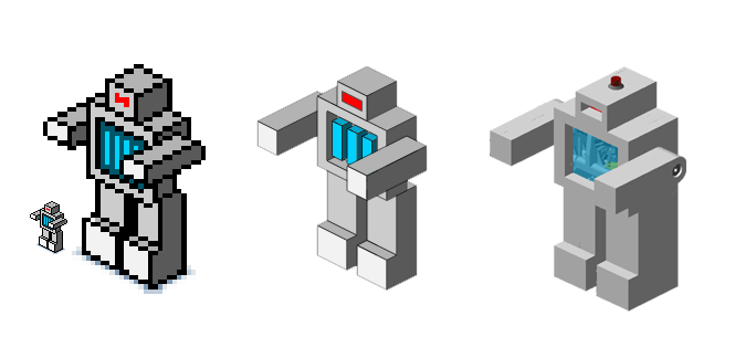
I searched for inspiration to figure out how I would tie all of these disciplines together. Growing up I read a lot of Sci-fi literature and a lot of that material stuck with me over the years, especially the portrayal of robots from the golden age. Above all, it captured the sense that anything was possible with technology and served as a great source of inspiration in my career. So without much surprise, I found the inspiration I needed for the project in my robot avatar. My mind was flickering with ideas as to how I could bring that simple icon to life and with that excitement I began my work.
Over the course of eight months I taught myself the necessary disciplines and skills to carry out my vision of building a simple 3D printed toy robot. Having finished my work at the end of July, I began compiling my notes and documenting my work and concluded this writing in the middle of October. This post is the culmination of that work and it will cover my technical work, thinking and experience. Above all, this is my story of bringing an idea to fruition while digging into the world of traditional engineering.
Outline
The scope of the project is fairly broad, so naturally, there’s a lot that I’m going to cover in this post. To help set some expectations on what you’ll encounter, I’m going to cover the three main stages of the project consisting of planning, building and evaluating; each covering the technical aspects related to industrial design, electronics and mechanics. In the planning section you can expect to read about the requirements, project plan and design of the product. In the building section, I’m going to cover the process of sourcing materials, prototyping and building the finished product. I’ll be wrapping up with a section dedicated to how the product was tested and some reflections on how I would approach the project again given the experience.
Related Work
While I was in the midst of doing some brainstorming last December I came across a series of YouTube videos by Jaimie Mantzel covering his experience building 3D printed toy hexapods. His “3D printed big robot” series really captured his enthusiasm and energy for the medium and while I wasn’t going to be making something as complicated as a hexapod, it was helpful to get a window into someone else’s mind and see how they approach the problem of making a product from scratch. Hopefully this document will inspire others to get out there and make something as much as these videos inspired me to do the same.
Planning Phase
Requirements
I designed my avatar about ten years ago and in reflecting on how I illustrated it at the time I began to think about what it would do in the real world. For starters, I envisioned an illuminated eye and chest opening with the later glowing on and off. The second thing I envisioned was that the arms would be able to swing back and forth opposite to one another giving the illusion of body language depending on the initial position of the arms: straight down giving the impression of marching, forward as though it were in a zombie state, all the way up as though in a panic and flung backward as though it were running around frantically. In short a variety of different personas.
Implicit to these behaviors are some underlying requirements. The toy requires power, so it makes sense to provide an on-off button somewhere on the design that is easy at access while the arms are in motion. Since the arms are in motion, it’s begs the question of for how long are the arms swinging in each direction and how quickly. Finally there is the frequency at which the chest lights pulsate on and off and with what type of waveform. The physical enclosure would be required to enclose all of the electronics and hardware components and also provide a means of assembling the parts within the enclosure and then providing a mechanism for securely closing the enclosure.
Since we are talking about engineering it makes sense to have a handful of engineering centric requirements. From an electronics engineering point of view, the components must be within their stated current and voltage tolerances as the power supply diminishes over time. From a mechanical point of view, the motor must supply sufficient torque to the mechanical system to ensure efficient transfer of motion to the arms so that the movement remains fluid, plus the product would need to be stable under static and dynamic loads. Finally, from an industrial design point of view, the product itself must be sturdy enough to withstand the forces that will be applied to it and be designed in a way that the fabrication process will yield a quality result.
Ultimately, we are talking about making a consumer product. That product needs to be polished in its appearance and stay true to the original avatar illustration. The product needs to be conscious of its life cycle as well in terms of being made from environmentally friendly components and practices, to being efficient in its use of energy and being capable of being recycled at the end of its life. As is the case with any project, there are a number of more nuanced requirements imposed by each of the components and tools used in the process of creating the product. I will discuss along the way how these constraints affected the project.
Methodology
Thinking about how to approach the project, I thought about how I’d approached projects of similar size and scope. My approach typically follows the iterative and incremental development methodology; do a lot of up front planning, cycle through some iterations and wrap up with a deployment. Rinse and repeat.
 |
In the introduction I talked about my thought process and motivation that constituted the brainstorming that was done to generate the requirements. From these requirements, I broke the problem down into smaller more digestible components that I could research and learn the governing models that dictate how those components behave from a mathematical point of view and on the computer through simulations. With that understanding, it was possible to put together a design that fulfills a specific set of conditions that result in the desired set of outputs. This design is the cornerstone of the initial planning.
The bulk of work is based in working through iterations that ultimately result in working components based on the design that was produced in the planning stage. Each iteration corresponds to a single component/requirement that starts off with building a prototype. For electronics this is done by prototyping on a breadboard, mechanics and industrial design with cardboard elements. The result is a functioning prototype that is used to create a refined design for the component that is then built. For example, a soldered protoboard or 3D printed volume. A completed component is tested and if accepted, stored for assembly.
As accepted components are completed, they are assembled into the broader view of the product. Each component is tested as part of the whole and if working correctly, fastened into place. Once all of the components are incorporated, the end product is tested and ultimately accepted. Throughout the process, if a particular output for an activity fails, then the previous activity is revisited until the root cause is identified, corrected and the process moves forward to completion.
Design
Industrial Design
Part Design
Knowing I didn’t know what I didn’t know about how to make a durable product, I did some research about part design and came across a set of design guidelines from Bayer Material Sciences covering the type of features that are added to products to make them more resilient to the kind of abuse consumer products are subjected to. This was helpful since it gave me a set of primitives to work with and in this project I ended up using a few of these features for providing strength to the product- ribs, gussets and trusses- and a few for allowing parts to be mated together- counterbores, taps and bosses.
 |
Ribs are used whenever there is a need to reduce the thickness of a plate and retain the plate’s original strength. When the thickness of the plate is reduced, so is the volume, and hence the cost but so too is the plate’s strength. To compensate, a rib is placed along the center of the plate and this increases the plate’s strength to its original state. A similar approach is deployed when talking about gussets as a way of providing added strength between two orthogonal faces. While not depicted above, the last technique deployed were trusses. Like what you’d find in the frames of your roof, the truss is a series of slats that form a triangular mesh that redistribute forces placed on the frame allowing it to take on greater load.
Counterbores are used so that the top of a machine screw sits flush or below the surface that needs to be fastened to another. The machine screws are then fastened to either a tap or a boss. A tap is a bored out section of material that is then threaded to act like a nut. Since we want to minimize material, the alternative is to carve out the material around the bore and leave a standing post that the machine screw will fasten to. Since the boss is freestanding, it may have gussets placed around its perimeter depending on the boss’s height.
Modeling
The first step in getting the 3D model put together was to use the pixel art version of my avatar to create a vectorized version for the purpose of developing a system of units and measurements that I could then use to develop a 3D model of the product in OpenSCAD. After having a chance to learn the software and its limitations, I set out to create a series of conventions to make it easy to work with parts, assemblies, enclosures in a variety of units and scales. Since real world elements would factor into the design of the product, I included all of the miscellaneous parts into the CAD model as well to make it easier to reason about the end result. After about a month of work the model was completed, let’s take a look at how it all came together.
The product consists of two arms, body, bracket and back plate. Each arm consists of a rounded shoulder with openings for fastening shaft collars; the shaft collars themselves and the shaft that extends from the body. The extended arm is hollow with interior ribs to add strength to the printed result. To support the printing process, small holes are added on the underside so that supporting material can be blown out.
On the exterior face of the back plate, the embossed designer logo, copyright and production number are provided to identify the product. Counterbores allow machines screws to be fastened to the main body at the base of legs and back of the head. On the interior face, the electronic components are fastened to bosses using machine screws. Since the back plate is just a thin plate, ribs were added to increase that plate’s strength.
The body has an opening on the top of the head for the on-off switch, and the face an opening for the eye plate and on the chest an opening for the chest plate. Counterbores line the hips so that machine screws can be fastened to the bracket to hold it in place. On the interior, horizontal bosses mate with counterbores on the back plate and several trusses and ribs were added to provide strength.
 |
A shelf separates the eye cavity from the chest cavity so that illumination from one doesn’t interfere with the other. Under the interior of the shoulders are the RIC for the material, WEEE logo, and along the leg, text describing the product with title, designer, date and copyright.
Finally, the bracket consists of two flanges with openings for ball bearings and a main shelf with an opening for the motor and set screws to secure the motor. The bracket has four taps that mate with the counterbores along the hip of the body.
Analysis
While I had a set of guidelines on how to make the product durable, most of the modeling process was more art than engineering. Since the 3D printing process would be fairly expensive, I wanted some additional confidence that the result was going to come out sturdy, so I thought a bit about it from a physics point of view. I knew of stress-strain analysis and that to understand how a complex object responds to loads I would need to use a Finite Element Analysis (FEA) solver on the 3D model. I researched the subject a bit, and once I felt I had a working understanding, I decided to use CalculiX to perform the actual computations. This section will cover the background, process and results at a very high level.
Stress-Strain Analysis
When a physical body is put under load, the particles of the body exert forces upon one another; the extent of these internal forces is quantified by stress. When the load begins to increase beyond the material’s ability to cope, the particles may begin to displace; how much they move about is quantified by strain.
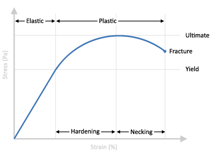 |
For small amounts of strain the material will behave elastically; returning to its original form once any applied forces are removed. As the amount of strain increases, and consequently the stress past the yield stress, the material begins to behave plastically; first hardening and then beginning to neck (i.e., thinning and separating) until it finally fractures. The specific critical values will depend entirely on the material and in this project an isotropic material, Polyamide PA 2200 (Nylon 12), will be used in the 3D printing process.
For a durable product, we obviously want to avoid subjecting the body to any forces that will result in permanent deformation which means keeping stress below the yield stress and even lower from an engineering point of view. The acceptable upper bound is given by a safety factor that linearly reduces the yield stress to an acceptable level. According to the literature a safety factor in the range ![N \in [1.1, 1.5]](https://s0.wp.com/latex.php?latex=N+%5Cin+%5B1.1%2C+1.5%5D&bg=ffffff&fg=1c1c1c&s=0&c=20201002)
To establish a design criteria, I went with a safety factor of 


Linear Stress-Strain Relationship
Given that we want to stay within the linear region, we can now begin to look at the specific relationship between stress, 


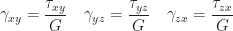
Both stress and strain are second-order tensors that relate how each of the three bases of a coordinate system relates to one another. When acting in the same dimension, the result is normal stress, 


Since we are working with an isotropic material, the resulting equations can be simplified to the following:

| Characteristic | Description | Polyamide 2200 Values |
|---|---|---|
| Young’s modulus | Slope of the stress-strain curve in the linear region. |  |
| Poisson’s ratio | Measure of how much a material will reduce as a consequence of being stretched. |  |
| Shear modulus | Function of the previous two and quantifies how force is needed before the material begins to shear. | 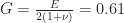 |
Finite Element Method (FEM)
To determine the stress and strain of a body under load we’ll rely on the FEM, a general purpose numerical method for calculating the approximate solution to a boundary value problem whose analytic solution is elusive. The general idea is that the problem domain can be broken into smaller elements, each analyzed individually, and the corresponding analyses combined so that an overarching solution can be determined.
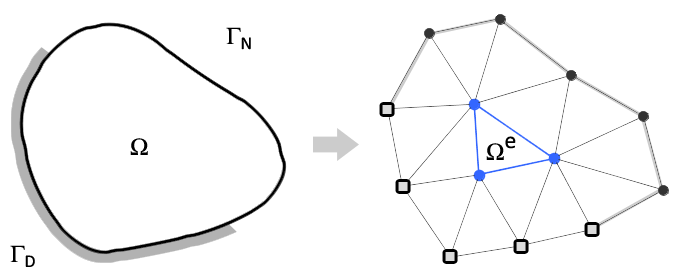 |
In the discretization step, the exact elements depend on the nature of the problem being solved, and in the case of stress analysis, into (linear or quadratic) tetrahedral elements consisting of nodes, edges and faces. In general, the nodes are being subjected to (unknown) internal and (known) external forces and the displacements of the nodes are to be determined. The relationship between the two is assumed to be linear. Thus, the following equation characterizes the state of the physical model at the element.

Where 


Standard algorithms such as Gaussian Elimination and the Gauss-Seidel Method can be used to solve for the displacement vector. With the displacement vector, stress and strain can then be computed at the nodes and interpolated across each element to produce the desired stress analysis. As the number elements increases, the error between the exact and approximate solution will decrease. This means that the FEM solution serves as lower bound to the actual solution.
Tool Chain
 |
Given the theory, it’s time to assemble the tools to carry out the job. The abundance of free computer aided design (CAD) and engineering (CEA) software made it easy to narrow down the options to OpenSCAD to define the geometry, MeshLab to clean the geometry, Netgen to mesh and define boundary conditions, and finally CalculiX to perform the necessary calculations and visualize the analysis. While each tool is excellent at carrying out their technical tasks, they are less polished from a usability point of view so additional time was spent digging under the hood to deduce expected behavior. Given the extra time involved, it’s worth covering the steps taken to obtain the end results.
The geometry of the product was modeled in OpenSCAD using its built-in scripting language. To share the geometry with Netgen, it is exported as a Standard Tessellation Language (STL) file which consists of a lattice of triangular faces and their corresponding normal vectors. Sometimes I found the exported STL file from OpenSCAD would cause Netgen to have a hard time interpreting the results, so MeshLab was used to pre-process the STL file and then hand it off to Netgen.
Netgen is used to load the geometry, generate the mesh and define boundary conditions. Once the geometry is loaded and verified with the built-in STL doctor, the engine is configured to generate a mesh and the process (based on the Delaunay algorithm) is carried out. Once the resulting mesh is available, the faces that correspond to the boundary conditions are assigned identifiers so they can be easily identified in CalculiX. The end result is exported a neutral volume file that CalculiX will be able to work with.
CalculiX consists of two components: GraphiX (CGX) and CrunchiX (CXX). CGX is used as a pre-processor to export the mesh in a format (MSH) that CCX can easily interpret, and specify and export the boundary conditions consisting of the fixed surfaces (NAM) and load conditions (DLO). CCX takes a hand written INP file that relates the material properties, mesh, and boundary conditions to the type of analysis to perform and then CCX carries out that analysis and outputs a series of files, most notably, the FRD file. CGX is then used as a post-processor to visualize the resulting stress and deformation results.
Finite Element Analysis (FEA)
The completed product will have pressure applied to the top of the head whenever the pushbutton is pushed to turn the product on or off; based on the design criteria, a uniform static pressure of 
Six configurations were run in order to evaluate the designs consisting of three mesh granularities against the model before and after strengthening enhancements were introduced. For the purpose of the analysis, it is assumed that the eye, chest and back plate are fixed to the body.
 |
Looking at the plots, the maximum displacement is centered about the through hole for the pushbutton which is consistent with one’s intuition. It appears that stress is most concentrated along the front where the head meets the shoulders and along the rim of the through hole for the pushbutton which matches up with the literature. After enhancements were introduced, it appears that displacement was reduced and that stress became more concentrated. Quantitatively:
| (Enhancement) | (Mesh Size) | Stress (MPa) | Displacement (mm) | ||
|---|---|---|---|---|---|
| Min | Max | Min | Max | ||
| Before | Moderate | 0.0166 | 1.27 | 0 | 0.519 |
| Fine | 0.0109 | 1.83 | 0 | 0.888 | |
| Very Fine | 0.00151 | 5.99 | 0 | 2.01 | |
| After | Moderate | 0.000648 | 2.5 | 0 | 0.631 |
| Fine | 0.000348 | 5.06 | 0 | 1.11 | |
| Very Fine | 0.000148 | 11.2 | 0 | 1.75 | |
After collecting the extremum from the test cases, the stress results seemed spurious to me. It didn’t feel intuitively right that applying a large amount of pressure to the head would result in at most a half of that pressure appearing throughout the body. I am assuming that there was a mix-up in the order magnitude of the units somewhere along the way. If the calculations are correct, then everything will be well below the yield stress and the product will be able to support what seems like a lot of stress. On the other hand, if the numbers are wrong, then I can’t make any claims other than relative improvements in the before and after; which was the main reason for carrying out the analysis.
From the literature, a finer mesh (i.e., a greater number of nodes) results in more accurate results. Looking at the outcome of the “Very Fine” mesh shows that the maximum stress in the product after enhancements is greater than the maximum stress before changes. However, the product is more rigid after the enhancement and admitted a reduced maximum displacement. This seems like an acceptable tradeoff since the goal was to make a product sturdier through enhancements.
Mechanics
Construction
 |
The next step in completing the design of the product was to focus on how to make a machine to rotate the arms. Not knowing a whole lot, the first step was to read up on the established elements and to think how they could be used to fulfill my needs. Out of this reading I came across the differential and how it was configured to rotate shafts at different speeds. Deconstructing the mechanism down to its primitive components enabled me to see how I could borrow from that design to come up with my own.
Gearmotor
At the heart of the mechanical system is a 100:1 (gear ratio) gearmotor consisting of a direct current (DC) motor and a gear train. For every rotation of the output shaft, the motor’s shaft rotates 100 times. This is achieved through the arrangement of gears in the gear train attached to the DC motor’s shaft. Since torque is proportional to the gear ratio, this means we get greater mechanical advantage.
Gear Train
The gearmotor is used to drive a gear train consisting of three gears: a pinion gear attached to the shaft of the gearmotor and two bevel gears that are perpendicular to the pinion. As the pinion gear rotates clockwise (resp. counterclockwise), one of the bevel gears will rotate clockwise (resp. counterclockwise) and the other will rotate counterclockwise (resp. clockwise). The pinion gear and bevel gears that will be used are in ratio of 1.3:1.
Shaft Assembly
To fix elements to the shaft, shaft collars are used to pinch the element into place along the shaft and each shaft collar is then fastened to the shaft using screw sets to retain the position and inward pressure on the element. Each bevel gear is connected to a shaft that extends outward to an arm. The main elements fastened using the sandwiching technique are the bevel gears, radial ball bearings that mesh with the bracket and body, and the arm. Outside the body, a spacer is used to displace the arm from the body and openings exist in the shoulder of the arm to access the shaft collars used to secure the arm.
Bracket
A modified clevis bracket will be used to hold the mechanical elements in place. The bracket consists of an opening in the middle to house the gearmotor along with two set screws openings to fasten it in place. To allow the bracket to be fitted with the body, machine screws are tapped along the edges of the bracket. Along the flanges of the bracket are openings for the radial ball bearings and each flange are supported by gussets to ensure that they don’t easily break off.
Analysis
Since we want to control the output of the arm as much as possible, we’ll want to explore how the arms behave at different orientations. To do so, we’ll assume that no external forces (with the exception of gravity) are acting on the arm and that the motor we are using a permanent magnet, direct current motor with a gearbox, specifically the KM-12FN20-100-06120 from the Shenzhen Kinmore Motor Co., Ltd. There are three views of the model that we’ll take into account: the arm, and the motor’s physical and electrical characteristics. Each view of the model will be presented, and then used to answer two questions (1) are there any orientations of the arm that cannot be supported by the motor and (2) are there any orientations that the motor cannot accelerate up to in order to achieve a steady angular velocity.
Arm
 |
While the geometry of the arm is more complex than a standard geometric primitive, it will be modeled as a cuboid with square edge length of, 


Since we are talking about rotating the arm, the moment of inertia will come into play. We’ll use the standard formula for a cuboid, superposition principle to account for the hollow interior and parallel axis theorem to deal with the pivot about the elbow in order to come up with the actual moment of inertia for the model, 
Physics
We have a series of torques being applied to the arm: first from the motor itself, 


The torque from the motor, 


The viscous friction, 

Torque due to gravity, 


Electronics
The ideal electronic model of the motor system is a series circuit consisting of the voltage, 


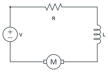 |
By Kirchhoff’s voltage law, the voltage applied to the terminals is equal to the sum of the potentials across each of the components giving:

The three constants in the equation, 

Since the resistance and inductance are not listed on the datasheet for the motor and could not be located online, we’d have to purchase the motor and then experimental determine their values. To complete the analysis, we’ll make simplify assumptions to work around this limitation.
Completed Model
Rewriting the physical and electronic governing equations in terms of the angular velocity, 

In doing so, we’d uncover nonlinear transient behavior and steady state fixed values that both current and angular velocity will approach in the limiting case.
Now that we have a complete model, we’ll make some simplifying assumptions in order to resolve questions (1) and (2). First, we’ll assume that the viscous friction constant is several orders magnitude smaller than the other terms and can be set to zero. Second, we’ll assume that the motor has accelerated up to a fixed angular velocity. Finally, we’ll assume the motor will always be supporting the worst case load from the arm. Under those assumptions we arrive at:

To approach question (2), let’s think about the current side of the system. The maximum current takes place when the motor shaft is not rotating. Using an ohmmeter to determine the terminal resistance, 


However, when we go to reverse the motor, we’ll introduce a drop from the steady state speed down to zero and then ramp back up in the opposite direction. So in reality, we may observe current changes on the order of twice that of 


Electronics
The final step in completing the design was to focus on how the electronics would illuminate the eye and chest cavity and drive the rotation of the arms. Being the main focus of the project, I will be covering how the electronics fulfill these requirements in a bit more depth than the two prior sections.
Motor Control
The motor control subsystem is responsible for managing how frequently and how quickly the motor needs to rotate in each direction. The subsystem consists of a timing circuit determining how frequently the motor will rotate, a pulse width modulated circuit to determine how quickly, a Boolean logic circuit to form composite signals that will be feed to a motor driver, and an H-Bridge circuit serving as the motor driver used to drive the gearmotor.
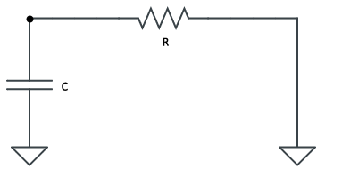
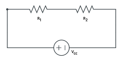
Series Resistor-Capacitor (RC) Circuits
To understand the basis for timing we’ll need to discuss series resistor-capacitor circuits briefly. Assume a series circuit consisting of a voltage source, 
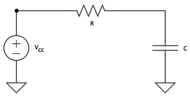
In the first, the capacitor will begin to charge allowing some of the current to pass through and then, once fully charged, it have such impedance that no current will flow through. Kirchhoff’s voltage law says that the voltage across the resistor and capacitor is equal to the supply voltage.

Since there is one path for current to flow through the entire circuit, the amount of current flowing through the resistor is the same as the capacitor. Using Ohm’s law and the definition of capacitance and current we arrive at an initial value problem consisting of a linear ordinary differential equation that can be solved using the technique of integrating factors.

Solving for equation we get a curve that grows with exponential decay and in the limiting case, approaches 


In the case of the discharging capacitor, Kirchhoff’s voltage law says the voltage of the capacitor is equal in magnitude to the voltage across the resistor.

Making the same assumptions as before, we arrive at another initial value problem consisting of a linear ordinary differential equation that can be solved using its characteristic equation.

As a result we get a curve that declines with exponential decay that will eventually approach zero in the limiting case. Using the timing constant again, we arrive at the following curve.

Timing
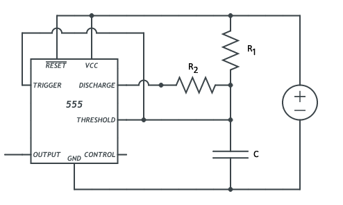 |
In order to tell the motor how long it needs to be on in one direction, a 555 integrated circuit is used to generate a square waveform of a fixed frequency. This is done by chaining a RC circuit with the inputs of the integrated circuit in astable mode to generate a 50% duty cycle waveform. The duty cycle is a way of measuring what percent the resulting square wave will spend in a high state relative to the period of the waveform. Here, we’ll have equal parts high state and low state each period.
 |
When an input voltage of one third that of the reference is applied to the trigger input, the output of the integrated circuit will be the same as the reference voltage. When two thirds the reference voltage is applied to the threshold input, the output voltage goes to ground. In this set up, the capacitor in the circuit will be continuously charging until the ceiling has been hit and then discharge until the floor and so on.
| Characteristic | Time (seconds) |
|---|---|
| Initial ramp up time |  |
| Discharge times | 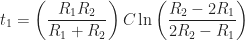 |
| Subsequent charge times |  |
| Period |  |
| Frequency |  |
| Duty cycle |  |
To calculate the values for 


Pulse Width Modulation (PWM)
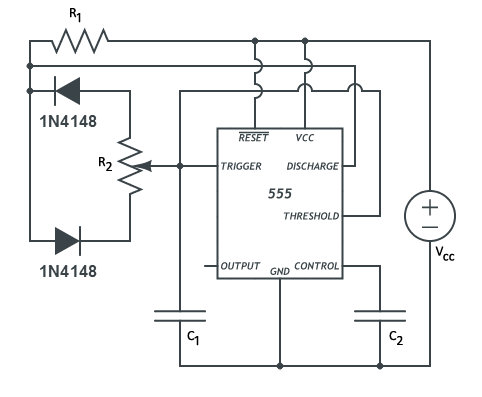 |
In order to control how fast the motor rotates, we’ll take advantage of the fact that the motor’s speed is linearly proportional to the voltage supplied to the motor and that the average output voltage of a PWM signal is linearly proportional to its duty cycle. To realize that plan, a 555 integrated circuit in astable mode is used to generate a high frequency signal whose duty cycle is controlled by the use of a potentiometer.
The fundamental operation of the 555 integrated circuit remains unchanged, however, the PWM circuit has a different topology than the timing circuit’s and as a result, has different timing characteristics. When the circuit is initially charging, current will go through 


Using values of 


| Characteristic | Time (seconds) |
|---|---|
| Initial ramp up time |  |
| Discharge times |  |
| Subsequent charge times |  |
Thus, we’ll end up with a circuit running at 

NOT-Gates and Resistor-Transistor Logic (RTL)
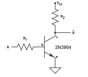 |
To begin talking about the logic used to combine the PWM and timing signals, we’ll need to perform negation of a signal, 


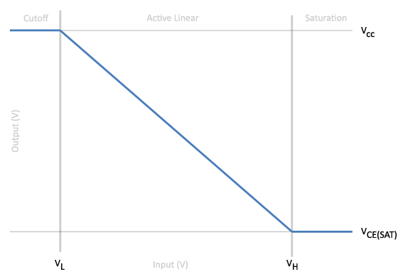
To determine the values of the resistors, we’ll need to look at the low-frequency, large signal model of the transistor which consists of three states: cut-off, active-linear and saturation. For the logic gate, we’ll want to minimize the active-linear region and focus on flip-flopping between the cut-off and saturation regions based on the value of
For the output to be logically true, 

If however, the input voltage is greater than 
 .
.Based on the condition that the ratio of the collector current and base current be less than the gain, 

 |
Given the latest piece of information, it’s possible to decide on a value of one resistor and pick the value of the other such that the collector resistor is several times larger than the base resistor and greater than 


Logic
 |
Given the timing signal and the PWM signal, we’ll produce a composite signal that will retain the period of the timing signal while controlling the observed amplitude from the PWM signal. This will give a signal that can be used to control one of the terminals of the gearmotor. Since the gearmotor terminals are designed to have one be in a ground state while the other in a high state, there will be a second composite signal that is simply the composite of the negation of the timing signal with the PWM signal.
 |
Since there were multiple signals to conjoin, I opted to use the 7408 quad, two-input AND-gate integrated circuit based on Transistor-transistor logic (TTL), a more efficient way of approaching the problem. I could have just as well used RTL to perform the conjunction, but the protoboard real estate required exceeded what I’d allocated and it simplified the design. There were NOT-gate integrated circuits that I could have used as well (e.g., 7404), but I decided to use the RTL based solution since it gave me an opportunity to learn the basics of transistors which would be required to understand the motor driver.
Driving the Motor
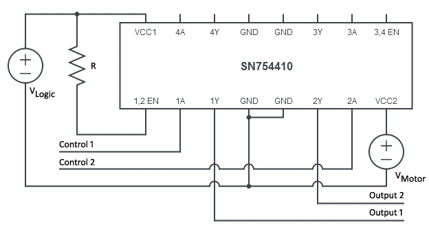 |
With the motor controller specified, it’s time to look at the motor driver. The gearmotor will draw a fair amount of current and since most of the logic circuitry is designed for low current consumption, it’s not feasible to drive the motor using the controller. Instead, an H-Bridge will be used to supply enough current while isolating the controlling logic.
An H-Bridge consists of several transistor switches and fly back diodes for controlling the flow of current. The motor is designed to rotate clockwise or counterclockwise depending on the polarity of the charges applied to the terminals. Since we’ve got two signals that designate which terminal is ground and which is high, it’s a matter of feeding the signals to the inputs of the bridge that correspond to rotating in the desired direction.
I’d put together two designs, one using bipolar junction transistors (BJT) and one using the SN754410 quadruple half-H-bridge integrated circuit. The first required a handful of components and wanting to better understand transistors, I opted to go this route for prototyping. In creating the production protoboard I decided to go with the SN74410 for reason’s I’ll cover in that section. As far as the design is concerned, they are functionality identical for exposing a higher voltage source to a motor while insulating the lower voltage controller circuitry.
Completed Motor Controller
 |
With a full list of schematics for the motor controller, the next step is to design the circuit that will be soldered to the controller’s protoboard. The motor controller will sit in one of the legs of the product and reside on a 
LED Control
Overall, the product consists of a single red LED for the eye, three blue LEDs for the chest and three green indicator LEDs used for debugging the circuit. The eye LED is always on, and a constant
Since the triangle oscillator represents the bulk of the circuit, this section will be dedicated to its analysis, operation and characteristics.
Voltage Divider
Since we’ll be using a single supply operational amplifier design to control the chest LEDs, we’ll need to create a reference voltage between the supply and ground. This will be achieved using a voltage divider. By Kirchhoff’s voltage law we have 

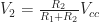


Non-inverting Schmitt Trigger
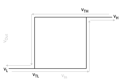 |
In the timing section we focused on creating a square wave output using a 555 timer. While this is one way to go about it, another is to use an operational amplifier based non-inverting Schmitt Trigger. The idea is that for a given voltage input, 


 |
In this configuration, the operational amplifier is used as a positive feedback loop, in which case there are two defining characteristics of its ideal behavior: (1) the output voltage of the amplifier, 


There are two cases to explore, in the first, we’ll assume 


On its own, the circuit won’t generate a square wave, but as the input varies with time, the circuit will flop-flop between ground and the supply voltage. The timing of which will be determined in part by the circuit’s noise immunity, i.e., the difference between the thresholds.
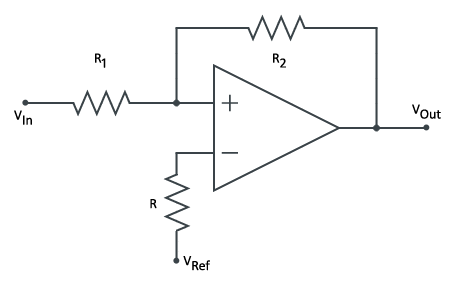
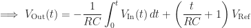
Inverting Integrator
 |
To complete the triangle oscillator, we’ll need to review the inverting integrator based on an operational amplifier. The idea behind the circuit is that as the input voltage varies with time, the output voltage will be the negated accumulation of that input.
The inverting integrator is an example of a negative feedback loop. The characteristics that applied to analyzing a positive feedback loop also apply to analyzing a negative feedback loop with the additional characteristic that (3) the voltage of the two terminals is identical, 
Par for the course, we’ll start by applying Kirchhoff’s current law to the inverting terminal of the operational amplifier.


Let’s assume that the input voltage can only take one of two values 


When
Triangle Oscillator
 |
Now that the Non-inverting Schmitt Trigger and Inverting Integrator have been covered, it’s time to loop the two together so that the trigger’s output feeds into the integrator’s input and its output into the trigger’s input. Assuming that when the circuit is started that the trigger’s output is the high state, the input – and hence the integrator’s output- has to be greater than the trigger’s upper threshold. (The complementary set of events would take place if we had instead assumed that the trigger was originally outputting a low state.)
As the trigger’s output continues to be the high state, the inverting integrator’s output will linearly decrease over time. This output will continue to be fed back into the trigger until the trigger’s lower threshold is surpassed. Once this happens, the trigger’s output will be the low state. As the trigger’s output continues to be in the low state, the integrator’s output will linearly increase over time. This output will continue to be fed back into the trigger until the trigger’s upper threshold is surpassed. The trigger’s output will then be the high state and the whole cycle will repeat itself.
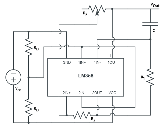 |
The completed circuit consists of a voltage divider, trigger and integrator around a LM358 dual operational amplifier. To provide a wide range of frequencies, I opted to use a potentiometer to control the frequency of the output rather than relying on a single fixed value resistor. This was done since I didn’t know what would be the ideal frequency and it bought me a range of solutions and not just one.
Based on the equations derived, the frequency and maximum outputs of the system are:

Using values of 


The design will use blue LEDs which come with a voltage drop of about 

Completed LED Controller
 |
All of the LEDs in the product in the chest cavity of the body and reside on a 
Power Control
In designing the electronics for managing the power in the product, I chose to provide two separate voltage sources: two AAA batteries giving a combined 

Of the subcomponents in the circuit, the boost converter is the most interesting; this section will be primarily devoted to discussing its analysis, operation and characteristics.
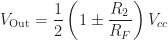
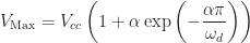
Series-Parallel Resistor-Inductor-Capacitor (RLC) Circuits
To begin talking about the boost converter, it’s necessary to talk about the series-parallel RLC circuit which differs from the standard series and parallel circuit topologies in that the inductor runs in series to a resistor and capacitor in parallel.
 |
While the topologies may differ, the characteristics used to simplify the analysis of RLC circuits remain the same. When convenient, the following substitutions will be made:
| Characteristic | Equation |
|---|---|
| Natural frequency |  |
| Dampening attenuation |  |
| Dampening factor |  |
| Dampened natural frequency |  |
Based on Kirchhoff’s voltage law the voltage source is the sum of the voltage across the inductor and that of the RC subcircuit. Kirchhoff’s current law says that the amount of current flowing through the inductor is the same as the aggregate current flowing through the capacitor and resistor. Based on these assumptions, we arrive at the following second order linear nonhomogeneous ordinary differential equation:

The general solution for a differential equation of this form is to take the superposition of the homogeneous solution with the particular (nonhomogeneous) solution. For the former we’ll use the characteristic equation of the homogeneous equation and then the method of undetermined coefficients for the latter.

Since we have a second order equation, we can run into repeated real roots (critically damped 


In order to determine the coefficients’ values, we’ll need to determine the initial conditions of the system. Initially, the inductor will resist any change in current, so since there is no current, the initial current is zero, 


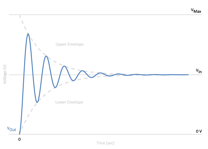 |
Looking at the voltage over time we see that the output voltage is greater than the input voltage at the beginning of the circuit’s uptime and as time elapses, the output voltage converges to the input voltage. The peak output voltage will be observed very early on at 
We’ll leverage this behavior to get the boost in voltage from the boost converter.
DC-DC Boost Converter
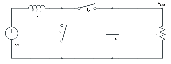 |
The boost converter is a way of converting an input voltage to a higher output voltage by switching between two different states that charge and discharge the inductor’s magnetic field. In the charging state, 


 |
For a thorough analysis of the boost converter, you should refer to Wens and Steyaert from which the following input-output voltage relationship is attributed.

As the duty cycle 
3V to 5V Boost Converter
To realize this boost converter design, I went with the Maxim MAX630 to serve as the first switch in the system and a 1N4148 diode to serve as the second switch. (The diode functions as a switch by only allowing current to move in one direction.) According to the Maxim datasheet, the MAX630 works by monitoring the voltage on VFB and when it is too low, the MAX630 oscillates its internal N-channel MOSFET at a high frequency open and shut on LX to put the system into the charging state. Once VFB is above the desired voltage, LX is left open to put the system into the discharging state. This cycle repeats until the system is powered off.
 |
Due to the oscillatory nature of the charging phase used by the MAX630, the analysis that was performed for the series-parallel RLC circuit is cumbersome to use here to determine the appropriate values for the passive components. Fortunately, the MAX630’s datasheet had a schematic for a 


Completed Power Controller
 |
The power controller will sit in one of the legs of the body and reside on a
Building Phase
Sourcing
 |
One thing that surprised me perhaps more than anything about this project was how difficult it was to find the right parts having the desired characteristics. Overall, I had orders with about a half dozen vendors from here in the United States and abroad.
3D Printing services were carried out by Shapeways, Inc. out of New York, New York. After receiving my package, I noticed a missing piece. After contacting their customer service they were able to resolve the matter and ship me a replacement part. Evidently since the missing piece was inside the main shell the operator didn’t see it on the reference, so it didn’t get shipped. The hiccup delayed me by about two weeks, but nonetheless, they made right by the mistake.
The Acrylic plates used on the front of the product were sourced from TAP Plastics of Mountain View, California. Painting supplies and adhesives and additional finishing tools were acquired from McGuckin’s Hardware store of Boulder, Colorado.
Machine elements were received from McMaster-Carr of Elmhurst, Illinois. They had quite possibility the fastest order placement to shipping time I’ve ever seen. I’d love to see the system that powers that operation. Additional elements were acquired from various Amazon merchants and local big-brand hardware stores. Gearmotor was purchased from Sparkfun Electronics of Boulder, Colorado.
Electronic components were primarily received from Mouser Electronics of Mansfield, Texas. Their selection and speed of shipping were superb. Additional components were purchased from electronics store J. B. Saunder’s of Boulder, Colorado when I needed something quickly and from various Amazon merchants.
In terms of cost of these parts, buying in bulk and in single orders saves on per item cost and on shipping. Buying just the components needed would have ended up being more expensive than buying them in bulk. In effect, multiple versions of the product could be produced cheaper than just producing one.
Prototyping
Industrial Design
 |
To develop a sense of how the product would come together, it was helpful to construct a cardboard based version of the final product based off the measurements I’d put together during the design phase. This enabled me to understand proportions, and the working space for the electronic and mechanical components. It also helped remind me that I was working towards a well-defined end goal.
Mechanical
As in the previous section, I also put together some cardboard based prototypes of the drive system. This consisted of a couple cardboard gears, a mocked up motor and a couple straws. Not being very savvy when it comes to all things mechanical, it was helpful to see the parts in action before committing to anything.
Once I had purchased the machine elements I wanted to see how the shafts and everything would mesh together so I decided to make a wooden version of the motor carriage. My thinking here was that if it was easy enough to make I could skip having that component 3D printed to save on cost. After a few trips to the lumber store, some careful drilling and wood glue, the motor carriage was put together and I was able to verify that the axle and motor assemblies would mesh together and be capable of reliably holding everything in place.
From this exercise I concluded that it wasn’t worth the extra effort to really spend a lot of time on the wooden version. I simply didn’t have the right tools or workspace to get the kind of precision that would be needed to make everything run smoothly so I proceeded to think about what the 3D printed version would look like.
Electronics
Working with the electronics was a bit of a steep learning curve to traverse, but as time went on, it became easier to translate circuit diagrams to the breadboard. Coming from a software background, I put together the circuits in as modular a way as possible to facilitate testing of sub circuits in isolation. This made it significantly easier than attempting to debug issues with the circuit as a whole.
Production
Industrial Design
 |
3D printing of the product was done by laser sintering. This is a process where a thin layer of ESA Polyamide 2200 is laid down and then the cross section of the product is heated to bond the material together with a new layer added and the process repeated until the volume is rendered.
After a month of modeling the product in OpenSCAD, the resulting STL file was submitted to be printed. After ten days, the product was fabricated and delivered. As an observation, the end result had a look and feel similar to that of a sugar cube. Overall, the detail on the product came out crisp and only those openings whose diameter was less than 2mm ended up coming out slightly deformed on one side. The rest of the details came out well. The back plate logo and copyright text as well as the interior WEEE symbol, RIC symbol and copyright text came out crisp and legible despite having fine details.
 |
From here, it was time to undertake the process of giving the exterior of the model an aluminum looking finish. This was achieved by applying an aerosol primer for plastics and several coats of a metallic paint that formed a firm film of enamel that added some extra strength to the body. In between coats, the body was sanded down with finer and finer grit to remove any imperfections or inconsistencies introduced during the spray paint process. I decided to keep the striations from the printing process since it gave the finished product a more believable brushed metal look. I didn’t paint the interior since I didn’t want any miniscule metallic flakes from the paint to potentially interact with the electronics.
 |
The acrylic for the eye and chest plate was cut by hand and seated into the body with an epoxy for binding acrylic to plastics. To give the chest plate the same look as the original illustration, several layers of electrical tape were placed on the back of the chest plate and the openings were cut out with an X-Acto knife. Each of the mechanical and electronic components that were part of the body was then secured with additional adhesives. To make sure the mechanical components lined up properly I threaded an aluminum shaft through the ball bearings and then glued each bearing to the body or bracket. Once the adhesive had dried, it was easy to slowly pull the shaft back out.
Mechanics
 |
The final production work on the mechanics dealt with securing the pinion gear to the motor shaft, motor to the chassis, bevel gears and machine elements to the shafts and finally securing the arms. One of the major complications in putting the mechanical system together was the fact that many of parts came from different vendors and possessed a mixture of imperial and metric units. As a result, things were done in more of a roundabout way than I would have liked to realize the original design. C’est la vie.
Starting with the gears themselves, the bevel gear had racetrack shaped interior diameter of about 4mm. The closest aluminum dowel that would fit was 5/64” in diameter. Being a nonstandard imperial diameter, I went with a 3/16″ diameter rod since it was a more prevalent diameter among the hardware vendors. To compromise, the bevel gears were attached and centered to the 5/64” dowel with adhesive and left to set. Once set, they were then placed and centered inside the 3/16″ rod and fixed with adhesive.
The pinion gear and the motor’s shaft both had a 3mm radius, but the shaft was D-shaped since it was intended to mate with a RC car wheel. (Coincidentally, the gears were part of a larger differential gear set intended for a RC car.) Despite the mismatch, the pinion and motor shaft shared the same diameter, so it was easy to secure the pinion on the shaft with adhesive.
You’ll note that fewer shaft collars were used as a consequence of this complication which was primarily rooted in my choice of gears. I didn’t have many options when it came to gears, and I went with the best of my worst options since it was cheaper to purchase the gears as a set, than it was to go out and buy all the gears individually for far more than I was willing to pay. Nonetheless, everything came together within reason.
Electronics
 |
Transcribing each portion of the prototype from the breadboard over to the protoboard was a challenge that lasted for a few months. I’d spent a fair amount of time and was becoming fatigued by the experience and had hit a low point in terms of morale and motivation. As a result, I made mistakes that I shouldn’t have been making and I recognized I needed to change what I was doing if I was going to finish the project. After taking a two week break and thinking I’d gotten things under control by double and triple checking my designs and taking my time to make sure I wasn’t putting parts in backward or offset or connecting parts together that shouldn’t be by accident, I ran into a major problem.
I could not identify a short in my original BJT based H-bridge design. After reviewing the protoboard layout, breadboard layout, the design, my reference material and datasheets, I was stumped. This went on for weeks and I realized that this was just something more involved to get right that I had led myself to believe and that I needed to move on. As a result, I compromised on the design and decided to use a quad half H-bridge integrated circuit in place of a BJT based H-bridge design.
I also concluded that I needed to change my approach to the power management for the project. I felt that drawing current from a single voltage supply for both the logic and drive wasn’t the right thing to do and that I need to split these concerns into their own dedicated voltage supplies. Not wanting to just throw another
In retrospect it wasn’t the right decision since it meant adding complexity to the end result. It also meant desoldering a lot of work and spending additional time and money on new parts and a new design. But at this point, I had committed to the change and proceeded. After receiving the new parts I went through another round of testing on the new designs on the breadboard and concluded that the changes would work and proceeded to solder the changes to the protoboards.
Ironically, the boost converter and quad half H-bridge integrated circuit were the easiest things to map to the protoboard and any doubt that I could not get the final electronics to work were gone. Despite the big change and the frustration, I felt hat I had turned things around and was back on track.
Having finished the protoboards I fastened them to the back plate and made sure there was enough room in the body for everything to fit. I’d given myself some room between the machinery and the electronics, but not enough for the wires to lie in between. With some electrical tape I was able to bind the wires tightly and secure everything in its place and was finally ready to test drive the end result.
Evaluation Phase
Testing
Having put so much effort into the body of the product, I didn’t really have the heart to subject the 3D printed bodies through any serious stress tests. In handling the material and developing a feel for it, I didn’t develop an impression that it was overly fragile; it withstood several rounds of aggressive sanding, boring and drilling without fracturing and warping. For me, this was good enough for something that would ultimately find a home on my bookshelf.
To identify any problems with the machinery of the product, I oriented the arms of the robot in to the various positions I talked about in the requirements section to see how it would behave. All the elevated orientations resulted in the arms swinging down then being driven by the machinery. I attribute this mainly to how the arms were fastened to the shaft by being pinched between two shaft collars and padded from the shaft with some electrical tape. In one sense this was good since it was putting too much strain on the motor, but on the other hand disappointing. Despite this complication, I decided that I was ok with just having the arms hanging down and shuffling back and forth.
The second big part of the character of the product was the illumination of the eye and chest. The eye ended up having plenty of light while the chest merely flickered on and off. Changing the power supply design and dimensions of the body resulted in a reduced voltage and increased displacement resulting in the diminished output. Since things were already soldered, I chose to leave things as is.
Future Work
The end result here isn’t without flaws. Working through the project I recognized along the way that there were things I hadn’t done quite right or that just didn’t sit with me well. The following is a list of things I would try to keep in mind next time I take on a project like this.
As far as the 3D printing process went, I would go back and redo how I incorporated the latching mechanism for the motor chassis and back plate. The biggest problem here was that post fabrication modifications had to be made since I incorrectly understood the tapping process. Nothing ruins precision faster than making changes by hand.
I had overlooked the theory behind illumination and had instead focused more on intuition. In the future I would spend more time reading up literature on the right amount of light to use based on what I wanted to illuminate and the different techniques that exist for providing different types of coverage. In retrospect, I think this would have given the end result a more polished look.
The mechanical work was complicated by the impedance between the imperial and metric standards of the parts involved. Part of this was poor planning on my part; part was difficultly finding the right parts at a hobbyist price point. Nonetheless, I’d like to continue to develop my understanding of mechanical systems and how they can be incorporated into electronically driven solutions.
I would have also incorporated some wiring management directly into the part so that it was less of a hassle to fit the back plate to the body with everything. I’d also switch to an existing cable management system instead of relying on screw terminals so that it was easier to snap things together and give the board a lower profile to save on space.
I’d like to explore printed circuit boards the next time I approach a project like this. My knowledge of circuit design going into this was limited, and it would have meant a lot of wasted time, material and money had I gone ahead and ordered PCBS this round. Given that I now have a working model to base future work, I would like to explore this route in the future.
As far as the on-off functionality goes, next time I think I will use a series of relays to switch access to the voltage supplies whenever a momentary push button is engaged. I think this would lead to a cleaner separation of the two voltage supplies.
The timing circuit was complicated by the initial ramp up time giving rise to a slow initial rotation until the threshold was reached to go in to astable mode. In the future I’d like to come up with a way to eliminate that initial ramp up from showing up in the output of the arms. Related to this, I’d like to be able to control the length of the timing pulses to swing between clockwise and counterclockwise rotations. In all likelihood, I’d use a microcontroller since it would give me the greatest range of flexibility.
Conclusion
With the finished product sitting on my bookshelf and reflecting on this project, the seasons it encompassed and the ups and downs I worked through, I have developed a greater appreciation for mechatronics, the physical product design cycle and the work people put into everyday products.
Taking the time to make something tangible for a change presented me with a number of challenges that I hadn’t had to face before and that’s what I enjoy most about these kinds of projects. It’s really about developing a new set of tools, techniques and thinking that I can apply to problems that arise in my personal and professional work.
This project allowed me to explore a number of interesting concepts within the framework of a seemingly simple toy. Let’s iterate over the main bullet points:
- Analog circuit design- complete analysis and use of passive components coupled with semiconductors with first real exposure to transistors, operational amplifiers and 555 timers.
- Protoboard design, soldering, debugging and desoldering techniques.
- Exposure to driving DC Motors using various techniques.
- Better understanding of hardware development and the product design process.
- Learned about industrial design guidelines and techniques for making cost effective products using 3D printed materials.
- Use of the finite element method to perform stress analysis of a complex geometric object. (Finally had an excuse to learn tensors.)
- Learned how to use an assortment of CAD, CAM and CAE software solutions.
Overall, the project produced a number of positive outcomes. As a stepping stone, this project has left me wanting to explore mechatronics more deeply and I’ve got a number of ideas brewing in mind that could lead to more advanced “toys” in the future. I feel confident that I can take the lessons learned from this experience and avoid pitfalls that I might encounter in more advanced projects of similar focus going forward. For now, those ideas will have to wait as I return to my world of code and numbers.
About the Author

|
Garrett Lewellen is a software developer working at a private start-up in the Denver Metro Area designing and developing SaaS-based systems. With eight years’ experience and formal education in computer science with emphasis in applied mathematics, his primary interests lie in the application of statistical models to problems that arise in general computing. When he’s not working on projects, he’s out exploring the Rocky Mountains and enjoying the great outdoors. |
Copyright
“3D Printed Toy Robot” available under CC BY-NC-ND license. Copyright 2013 Garrett Lewellen. All rights reserved. Third-part trademarks property of their respective owners.
Bibliography
Part and Mold Design. [pdf] Pittsburgh, PA: Bayer Material Science, 2000. Web.
“A.5.8 Triangle Oscillator.” Op Amps For Everyone Design Guide (Rev. B). [pdf] Ed. Ron Mancini. N.p.: n.p., 2002. N. pag. Texas Instruments, 22 Aug. 2002. Web.
“Boost Converter.” Wikipedia. Wikimedia Foundation, 09 July 2013. Web. 15 Sept. 2013.
“What Is PWM? Pulse Width Modulation Tutorial in HD.” Electronics Tutorial Videos. N.p., 28 Nov. 2011. Web. 11 Sept. 2013.
Amado-Becker, Antonio, Jorge Ramos-Grez, María José Yañez, Yolanda Vargas, and Luis Gaete. “Elastic Tensor Stiffness Coefficients for SLS Nylon 12 under Different Degrees of Densification as Measured by Ultrasonic Technique.” [pdf] Rapid Prototyping Journal 14.5 (2008): 260-70. Web.
Chaniotakis. Cory. “Operational Amplifier Circuits Comparators and Positive Feedback”. [pdf] 6.071J/22.071, Introduction to Electronics, Signals, and Measurement. Spring 2006 Lecture Notes.
Cook, David. “Driving Miss Motor.” Intermediate Robot Building. 2nd ed. Apress, 2010. N. pag. Print.
Cook, David. “H-Bridge Motor Driver Using Bipolar Transistors.” Bipolar Transistor HBridge Motor Driver. N.p., n.d. Web. 11 Sept. 2013.
EOS GmbH – Electro Optical Systems, “PA 2200”: [pdf] Material sheet, 2008.
Demircioglu, Ismail H. “Dynamic Model of a Permanent Magnet DC Motor”. [pdf] 11 Aug. 2007.
Jung, Walt, ed. Op Amp Applications Handbook. N.p.: Analog Devices, 2002. Web.
Kim, Nam H., and Bhavani V. Sankar. Introduction to Finite Element Analysis and Design. 1st ed. New York: John Wiley & Sons, 2009. Print.
Lancaster, Don. RTL Cookbook. [pdf] 3rd ed. Thatcher, Arizona: Synergetics, 2013. Web. 11 Sept. 2013.
Maksimović, Dragan. “Feedback in Electronic Circuits: An Introduction”. [pdf] ECEN 4228, Analog IC Design. Lecture Notes 1997.
Mantzel, Jamie. 3D Print Big Robot Project No. 1. N.d. Youtube.com. 11 Mar. 2012. Web.
Maxim, “CMOS Micropower Step-Up Switching Regulator”, [pdf] MAX630 datasheet, Sept. 2008. .
Movellan, Javier R. “DC Motors.” [pdf] 27 Mar. 2010.
National Semiconductor, “LM555 Timer,” [pdf] LM555 datasheet, July 2006.
Najmabadi, Farrokh. “Bipolar-Junction (BJT) transistors.” [pdf] ECE60L, Components & Circuits Laboratory. Spring 2004 Lecture Notes. .
Nikishkov, G.P. “Introduction to the Finite Element Method”. [pdf] 2004 Lecture Notes.
Platt, Charles. Make: Electronics (Learning by Discovery). 1st ed. Sebastopol, CA: O’Reilly Media, Inc., 2009. Print.
Roberts, Dustyn. Making Things Move DIY Mechanisms for Inventors, Hobbyists, and Artists. 1st ed. N.p.: McGraw-Hill, 2010. Print.
Sayas, Francisco-Javier. “A gentle introduction to the Finite Element Method”. [pdf] 2008 Lecture Notes.
Shenzhen Kinmore Motor Co., Ltd, “Outline”, [pdf] KM20100507 datasheet, Nd.
Texas Instruments, “LM158, LM158A, LM258, LM258A, LM358, LM358A, LM2904, LM2904V Dual Operational Amplifiers”, [pdf] LM358 datasheet, June 1976 [Revised July 2010].
Texas Instruments, “SN754410 Quadruple Half-H Driver”, [pdf] SN754410 datasheet, Nov. 1986 [Revised 1995].
Toledo, Manuel. “Basic Op Amp Circuits”. [pdf] INEL 5205, Instrumentation. Lecture Notes. 13 Aug, 2008.
Wens, Mike, and Michiel Steyaert. “Reflections on Steady-State Calculation Methods.” Design and Implementation of Fully-integrated Inductive DC-DC Converters. N.p.: Springer, 2011. N. pag. Print. Analog Circuits and Signal Processing.
MMXIII
With a new year comes some new thinking on the direction I’d like to take my work and consequently, the site. Since the site’s inception in 2008, I’ve attempted to follow a monthly publication format throughout the year with the usual summer hiatus. This approach has worked well in the past since most of my work consisted of weekend projects. As I’ve refined my capabilities, I’ve sought out more sophisticated interests and challenges to take on as projects and research opportunities. Naturally, these more advanced projects require more time to finish. As I think about the next year and beyond, I’m certain this trend will continue.
Humans are lousy at multitasking, working on multiple projects simultaneously starts to rapidly produce diminishing returns in quality of work. Since my projects will continue to grow in complexity, a monthly format will soon require that I work on dozens of projects in parallel. With each additional project, the amount of time I can dedicate to a project each month will diminish and each project will take progressively longer to complete. Consequently, I’ve decided that I’m no longer going to try and finish a project each month along with the associated monthly post, rather I’d like to focus on developing my project and research, and publishing by the maxim “it’s done when it’s done”.
I know many people in my position opt to publish progress reports for long standing projects. I’ve done this in the past and have always felt that it ended up requiring too much duplication without any real benefit and reading them always felt like reading an arbitrary page out of a piece of fiction- the context simply isn’t there and it simply isn’t interesting to read. With that in mind, I want to talk about what projects I am currently working on some projects that I’m considering approaching over the next year and beyond.
Last year I began working on a couple of Android projects, Viderefit and an unannounced platformer. Viderefit got out the door, and the platformer was stalled in its inception phase and I’ve been contemplating how it will come together on and off since then. This will be a larger programming project than the rest of the projects I have planned, but it will be a continuation of the work I’ve done in developing arcade games in years past. Since these larger programming projects are better suited for winter, beginning next year I will be focusing on this project in more detail. Similarly, I’ll be spending more time on Viderefit this upcoming spring as the weather here in Colorado starts to warm back up and my outdoor season begins.
For the past several years I’ve been responsible for designing and overseeing distributed processing systems. Much of what I’ve observed can be characterized mathematically as stochastic dynamical systems. I view this as an opportunity to take what I’ve learned in industry and to apply that knowledge to studying these systems more formally. Since last fall, I’ve been delving into the theory of stochastic processes and seeing how that theory corresponds to what I’ve observed in the field. My goal is provide a thorough analysis of these systems and under what conditions they are stable.
In an attempt to broaden the purview of my work, I’ve been exploring mathematical finance and its role in business. I’ve started writing an overview of stock and stock options from the point of view of all the parties involved- shareholders, members, the exchange, traders and so on. There is some overlap in the stochastic elements of my distributed processing systems research which I hope to apply here as well, in particular options pricing. Overall, the goal is to put together an accessible overview of the instrument suitable for developers.
Since the beginning of the year, I’ve been working on a 3D printed toy robot. The opportunity to combine art, electronics, and mechanics together was too good an opportunity to pass up. The focus is on combining multiple engineering disciplines to produce a tangible result. In particular, to explore the possibilities of 3D printing, get some exposure to designing simple analog circuits, and utilize rudimentary mechanical constructs to bring a simple toy robot to life. Due to the inherent complexities of the project, and prolonged logistics involved in sourcing electronics and mechanical materials, this project is anticipated to be finished before the end of the year.
In parallel to my work on distributed processing systems, I’ve spent time being involved in applying natural language processing to problems in the medical industry. This is one area that I see a lot of potential commercially and I think it is worthwhile to pursue the subject in greater detail. A couple of years ago I wrote about an interpreter framework and its use for evaluating sentential logic. I’d like to extend that work to predicate logic and soundness checking, and then applying that solution to evaluating the soundness of English text. I’m also interested in building a speech synthesizer that can mimic the voice of any speaker given ample training data and a Russian to English statistical translator.
My work this past fall on image processing and category recognition was a rewarding process. I’m currently interested in learning more about how I can augment the mobile computing experience with augmented reality, and in what ways that marriage can result in meaningful, practical solutions for end users, and not just something that satisfies some intellectual curiosity. Likewise, I’m interested in exploring how image processing and machine learning can be applied to interpret body language and other non-verbal communication.
I see the next year full of interesting projects and possibilities that I believe will broaden my understanding of several subjects and give me an opportunity to deepen my knowledge in areas where I’m already knowledgeable. The underlying themes here are exploring the fascinating possibilities that arise from the intersection of mathematics, computer science and business, and the theme of growth and continued pursuit of bigger and better intellectual challenges. We’ll see how the new format works out and whether or not it produces noticeably improved results by this time next year when I plan to revisit my progress on these projects.
Expected Maximum and Minimum of Real-Valued Continuous Random Variables
Introduction
This is a quick paper exploring the expected maximum and minimum of real-valued continuous random variables for a project that I’m working on. This paper will be somewhat more formal than some of my previous writings, but should be an easy read beginning with some required definitions, problem statement, general solution and specific results for a small handful of continuous probability distributions.
Definitions
Definition (1) : Given the probability space, 


- Non-negativity:
- Null empty set:
- Countable additivity of disjoint sets


Definition (2) : Given a real-valued continuous random variable such that 


Defintion (3) : Given a second real-valued continuous random variable, 


Definition (4) : Given a real-valued continuous random variable, 
Definition (5) : (Law of the unconscious statistician) Given a real-valued continuous random variable, 


Remark (1) : For the remainder of this paper, all real-valued continuous random variables will be assumed to be independent.
Problem Statement
Theorem (1) : Given two real-valued continuous random variables 

Lemma (1) : Given two real-valued continuous random variables
Proof of Lemma (1) :


Proof of Theorem (1)


Remark (2) : For real values 

Proof Remark (2) : If 


Worked Continuous Probability Distributions
The following section of this paper derives the expected value of the maximum of real-valued continuous random variables for the exponential distribution, normal distribution and continuous uniform distribution. The derivation of the expected value of the minimum of real-valued continuous random variables is omitted as it can be found by applying Theorem (1).
Exponential Distribution
Definition (6) : Given a real-valued continuous exponentially distributed random variable, 


Corollary (6.i) The cumulative distribution function of a real-valued continuous exponentially distributed random variable, 
Proof of Corollary (6.i)

Corollary (6.ii) : The expected value of a real-valued continuous exponentially distributed random variable, 
Proof of Corollary (6.ii)
The expected value is 

Lemma (2) : Given real values 

Proof of Lemma (2) :


Theorem (2) : The expected value of the maximum of the real-valued continuous exponentially distributed random variables 
Proof of Theorem (2) :


Normal Distribution
Definition (7) : The following Gaussian integral is the error function 
- Odd function:
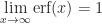
- Limiting behavior:

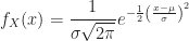
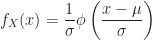
Definition (8) : Given a real-valued continuous normally distributed random variable , 


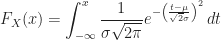
Corollary (8.i) : The cumulative distribution function of a real-valued continuous normally distributed random variable, 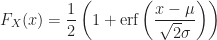
Proof of Corollary (8.i) :
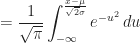


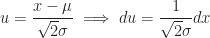
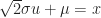
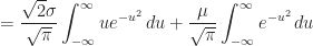
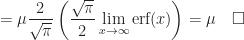
Corollary (8.ii) : The expected value of a real-valued continuous normally distributed random variable, 
Proof of Corollary (8.ii) :


Definition (9) : Given a real-valued continuous normally distributed random variable, 


- Non-standard probability density function: If
- Non-standard cumulative distribution function: If
- Complement:


Definition (10) : [PaRe96] Given


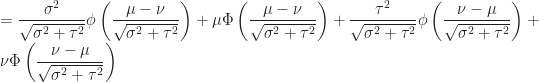
Theorem (3) : The expected value of the maximum of the real-valued continuous normally distributed random variables 
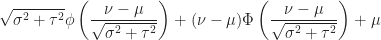
Lemma (3) : Given real-valued continuous normally distributed random variables 
Proof of Lemma (3) :

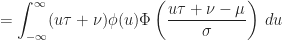


Proof of Theorem (3) :


Continuous Uniform Distribution
Definition (11) : Given a real-valued continuous uniformly distributed random variable, 


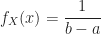
![x \in [a, b]](https://s0.wp.com/latex.php?latex=x+%5Cin+%5Ba%2C+b%5D&bg=ffffff&fg=1c1c1c&s=0&c=20201002)
Corollary (11.i) : The cumulative distribution function of a real-valued continuous uniformly distributed random variable, ![\displaystyle F_X(x) = \begin{cases} 0 & x < a \\ \frac{x-a}{b-a} & x \in [a,b] \\ 1 & x > b \end{cases}](https://s0.wp.com/latex.php?latex=%5Cdisplaystyle+F_X%28x%29+%3D+%5Cbegin%7Bcases%7D+0+%26+x+%3C+a+%5C%5C+%5Cfrac%7Bx-a%7D%7Bb-a%7D+%26+x+%5Cin+%5Ba%2Cb%5D+%5C%5C+1+%26+x+%3E+b+%5Cend%7Bcases%7D&bg=ffffff&fg=1c1c1c&s=0&c=20201002)
Proof of Corollary (11.i) :
![\displaystyle F_X(x) = \int_{-\infty}^{\infty} f_X(t) \, dt = \int_{a}^{b} \frac{1}{b-a} \, dt = \frac{1}{b-a} x \bigg|_{a}^{x} = \begin{cases} 0 & x < a \\ \frac{x-a}{b-a} & x \in [a,b] \\ 1 & x > b \end{cases}\quad \square](https://s0.wp.com/latex.php?latex=%5Cdisplaystyle+F_X%28x%29+%3D+%5Cint_%7B-%5Cinfty%7D%5E%7B%5Cinfty%7D+f_X%28t%29+%5C%2C+dt+%3D+%5Cint_%7Ba%7D%5E%7Bb%7D+%5Cfrac%7B1%7D%7Bb-a%7D+%5C%2C+dt+%3D+%5Cfrac%7B1%7D%7Bb-a%7D+x+%5Cbigg%7C_%7Ba%7D%5E%7Bx%7D+%3D+%5Cbegin%7Bcases%7D+0+%26+x+%3C+a+%5C%5C+%5Cfrac%7Bx-a%7D%7Bb-a%7D+%26+x+%5Cin+%5Ba%2Cb%5D+%5C%5C+1+%26+x+%3E+b+%5Cend%7Bcases%7D%5Cquad+%5Csquare&bg=ffffff&fg=1c1c1c&s=0&c=20201002)
Corollary (11.ii) : The expected value of a real-valued continuous uniformly distributed random variable, 
Proof of Corollary (11.ii)

Theorem (4) : The expected value of the maximum of real-valued continuous uniformly distributed random variables 

Proof of Theorem (4) :

![\displaystyle = \int_{a}^{b} x \frac{1}{b-a} \begin{cases} 0 & x < c \\ \frac{x - c}{d-c} & x \in [c,d] \\ 1 & \text{otherwise} \end{cases} \, dx + \int_{c}^{d} y \frac{1}{d-c} \begin{cases} 0 & y < a \\ \frac{y - a}{b-a} & y \in [a,b] \\ 1 & \text{otherwise} \end{cases} \, dy](https://s0.wp.com/latex.php?latex=%5Cdisplaystyle+%3D+%5Cint_%7Ba%7D%5E%7Bb%7D+x+%5Cfrac%7B1%7D%7Bb-a%7D+%5Cbegin%7Bcases%7D+0+%26+x+%3C+c+%5C%5C+%5Cfrac%7Bx+-+c%7D%7Bd-c%7D+%26+x+%5Cin+%5Bc%2Cd%5D+%5C%5C+1+%26+%5Ctext%7Botherwise%7D+%5Cend%7Bcases%7D+%5C%2C+dx+%2B+%5Cint_%7Bc%7D%5E%7Bd%7D+y+%5Cfrac%7B1%7D%7Bd-c%7D+%5Cbegin%7Bcases%7D+0+%26+y+%3C+a+%5C%5C+%5Cfrac%7By+-+a%7D%7Bb-a%7D+%26+y+%5Cin+%5Ba%2Cb%5D+%5C%5C+1+%26+%5Ctext%7Botherwise%7D+%5Cend%7Bcases%7D+%5C%2C+dy&bg=ffffff&fg=1c1c1c&s=0&c=20201002)
Case (1) :

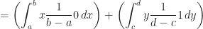

Case (2) :


Case (3) :


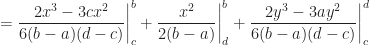


Case (4) :


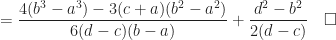
Case (5) :


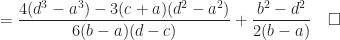
Case (6) :

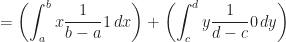

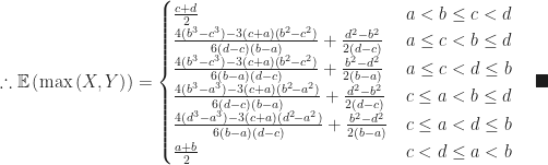
Summary Table
The following summary table lists the expected value of the maximum of real-valued continuous random variables for the exponential distribution, normal distribution and continuous uniform distribution. The corresponding minimum can be obtained by Theorem (1).
| Random Variables | Maximum | |
|---|---|---|
 |
 |
|
 |
 |
|
 |
 |
|
 |
 |
|
References
[GrSt01] Grimmett, Geoffrey, and David Stirzaker. Probability and Random Processes. Oxford: Oxford UP, 2001. Print.
[PaRe96] Patel, Jagdish K., and Campbell B. Read. Handbook of the Normal Distribution. 2nd ed. New York: Marcel Dekker, 1996. Print.
Parallel Merge Sort in Java
Introduction
This past November I was a pretty busy getting settled into a new job and trying to balance life’s other priorities. With a new job also came a new technology stack and while I’ll continue to do C# development in my free time, I’m going to be going back to doing Java development after a seven year hiatus. Before starting the new job, I decided to refresh my memory of the language’s finer details when it comes to generics and threading. So, I decided to implement something simple and settled on a parallel implementation of merge sort. This article is going to focus on making use of Java’s various features and evaluating the theoretical and empirical run time performance of the sequential and parallel versions of the algorithm.
Sequential Approach
Specification
Given a list of values, the list is sorted by employing a divide and conquer method that partitions the list into two (roughly) equal sized partitions, followed by recursively sorting each partition and then merging the two resulting sorted partitions into the final sorted list.
Pseudocode
![\displaystyle \textbf{MERGE}(X, Y) \newline \indent L_X \leftarrow \textbf{LENGTH}(X) \newline \indent L_Y \leftarrow \textbf{LENGTH}(Y) \newline \indent L_Z \leftarrow L_X + L_Y \newline \indent Z \leftarrow [L_Z] \newline \indent i, j, k \leftarrow 0, 0, 0 \newline \newline \indent \textbf{while} \quad k < L_Y \newline \indent \indent \textbf{if} \quad i < L_X \land j \ge L_Y \newline \indent \indent \indent \indent Z[k] \leftarrow X[i] \newline \indent \indent \indent \indent i \leftarrow i + 1 \newline \indent \indent \textbf{else-if} \quad i \ge L_X \land j < L_Y \newline \indent \indent \indent \indent Z[k] \leftarrow Y[j] \newline \indent \indent \indent \indent j \leftarrow j + 1 \newline \indent \indent \textbf{else-if} \quad i < L_X \land j < L_Y \newline \indent \indent \indent \textbf{if} \quad X[i] \le Y[j] \newline \indent \indent \indent \indent Z[k] \leftarrow X[i] \newline \indent \indent \indent \indent i \leftarrow i + 1 \newline \indent \indent \indent \textbf{else} \newline \indent \indent \indent \indent Z[k] \leftarrow Y[j] \newline \indent \indent \indent \indent j \leftarrow j + 1 \newline \indent \indent k \leftarrow k + 1 \newline \newline \indent \textbf{return} \quad Z](https://s0.wp.com/latex.php?latex=%5Cdisplaystyle+++%5Ctextbf%7BMERGE%7D%28X%2C+Y%29++%5Cnewline+%5Cindent+L_X+%5Cleftarrow+%5Ctextbf%7BLENGTH%7D%28X%29++%5Cnewline+%5Cindent+L_Y+%5Cleftarrow+%5Ctextbf%7BLENGTH%7D%28Y%29++%5Cnewline+%5Cindent+L_Z+%5Cleftarrow+L_X+%2B+L_Y++%5Cnewline+%5Cindent+Z+%5Cleftarrow+%5BL_Z%5D++%5Cnewline+%5Cindent+i%2C+j%2C+k+%5Cleftarrow+0%2C+0%2C+0++%5Cnewline++%5Cnewline+%5Cindent+%5Ctextbf%7Bwhile%7D+%5Cquad+k+%3C+L_Y++++%5Cnewline+%5Cindent+%5Cindent+%5Ctextbf%7Bif%7D+%5Cquad+i+%3C+L_X+%5Cland+j+%5Cge+L_Y++%5Cnewline+%5Cindent+%5Cindent+%5Cindent+%5Cindent+Z%5Bk%5D+%5Cleftarrow+X%5Bi%5D++%5Cnewline+%5Cindent+%5Cindent+%5Cindent+%5Cindent+i+%5Cleftarrow+i+%2B+1++%5Cnewline+%5Cindent+%5Cindent+%5Ctextbf%7Belse-if%7D+%5Cquad+i+%5Cge+L_X+%5Cland+j+%3C+L_Y++%5Cnewline+%5Cindent+%5Cindent+%5Cindent+%5Cindent+Z%5Bk%5D+%5Cleftarrow+Y%5Bj%5D++%5Cnewline+%5Cindent+%5Cindent+%5Cindent+%5Cindent+j+%5Cleftarrow+j+%2B+1++%5Cnewline+%5Cindent+%5Cindent+%5Ctextbf%7Belse-if%7D+%5Cquad+i+%3C+L_X+%5Cland+j+%3C+L_Y++%5Cnewline+%5Cindent+%5Cindent+%5Cindent+%5Ctextbf%7Bif%7D+%5Cquad+X%5Bi%5D+%5Cle+Y%5Bj%5D++%5Cnewline+%5Cindent+%5Cindent+%5Cindent+%5Cindent+Z%5Bk%5D+%5Cleftarrow+X%5Bi%5D++%5Cnewline+%5Cindent+%5Cindent+%5Cindent+%5Cindent+i+%5Cleftarrow+i+%2B+1++%5Cnewline+%5Cindent+%5Cindent+%5Cindent+%5Ctextbf%7Belse%7D+++%5Cnewline+%5Cindent+%5Cindent+%5Cindent+%5Cindent+Z%5Bk%5D+%5Cleftarrow+Y%5Bj%5D++%5Cnewline+%5Cindent+%5Cindent+%5Cindent+%5Cindent+j+%5Cleftarrow+j+%2B+1++%5Cnewline+%5Cindent+%5Cindent+k+%5Cleftarrow+k+%2B+1++%5Cnewline++%5Cnewline+%5Cindent+%5Ctextbf%7Breturn%7D+%5Cquad+Z++&bg=ffffff&fg=1c1c1c&s=0&c=20201002)
|

|
![\displaystyle \textbf{PARTITION}(X, s, L) \newline \indent Y \leftarrow [L] \newline \indent k \leftarrow 0 \newline \newline \indent \textbf{while} \quad k < L \newline \indent \indent Y[k] \leftarrow X[s + k] \newline \indent \indent k \leftarrow k + 1 \newline \newline \indent \textbf{return} \quad Y](https://s0.wp.com/latex.php?latex=%5Cdisplaystyle+++%5Ctextbf%7BPARTITION%7D%28X%2C+s%2C+L%29++%5Cnewline+%5Cindent+Y+%5Cleftarrow+%5BL%5D++%5Cnewline+%5Cindent+k+%5Cleftarrow+0++%5Cnewline++%5Cnewline+%5Cindent+%5Ctextbf%7Bwhile%7D+%5Cquad+k+%3C+L++%5Cnewline+%5Cindent+%5Cindent+Y%5Bk%5D+%5Cleftarrow+X%5Bs+%2B+k%5D++%5Cnewline+%5Cindent+%5Cindent+k+%5Cleftarrow+k+%2B+1++%5Cnewline++%5Cnewline+%5Cindent+%5Ctextbf%7Breturn%7D+%5Cquad+Y++&bg=ffffff&fg=1c1c1c&s=0&c=20201002)
Time Complexity
In terms of time complexity, the algorithm is on the order of 


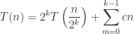
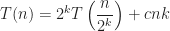


Implementation
In attempting to implement a generic version of merge sort there were a few matters that needed to be addressed. First, the type being sorted required an order relation to be specified so that the merge operation could take place. This is facilitated by restricting the type parameter T to Comparable<T>. Secondly, I had forgotten that you can’t initialize arrays of generics in Java like you can in C# [1]. To workaround this limitation, I settled on specifying the desired operations over implementations of the List<T> interface. Finally, since the List<T> interface makes no guarantees that its implementations provide (near) constant time reading or writing of elements from the list, an additional generic parameter, L, was added so that only those implementations of the List<T> and RandomAccess [2] interfaces could use this implementation of merge sort. The rest of the implementation is a near facsimile of the pseudocode.
package com.wordpress.antimatroid;

import java.util.List;
import java.util.RandomAccess;

public interface IListOperation
    <T, L extends List<T> & RandomAccess> {

	L execute();
}
package com.wordpress.antimatroid;

import java.util.ArrayList;
import java.util.List;
import java.util.RandomAccess;

public class CopyListOperation
    <T, L extends List<T> & RandomAccess>
    implements IListOperation<T, L> {

	private final L source;
	private final int length, initialIndex;

	public CopyListOperation(L source, int length, int initialIndex) {
		if(source == null)
			throw new IllegalArgumentException("source must be non-null.");

		if(length < 0)
			throw new IllegalArgumentException(String.format(
                "length, %d, must be greater than or equal to zero.", length
            ));

		if(initialIndex < 0)
			throw new IllegalArgumentException(String.format(
                "initialIndex, %d, must be greater than or equal to zero.", initialIndex
            ));

		if(initialIndex + length > source.size())
			throw new IllegalArgumentException(String.format(
                "initialIndex, %d, + length, %d, must be less than or equal to source.size(), %d.",
                initialIndex, length, source.size()
            ));

		this.source = source;
		this.length = length;
		this.initialIndex = initialIndex;
	}

	@Override
	public L execute() {
		L destination = (L) new ArrayList<T>(length);
		for(int i = 0; i < length; i++)
			destination.add(i, source.get(initialIndex + i));
		return destination;
	}
}
package com.wordpress.antimatroid;

import java.util.ArrayList;
import java.util.List;
import java.util.RandomAccess;

public class MergeListOperation
    <T extends Comparable<T>, L extends List<T> & RandomAccess>
    implements IListOperation<T, L> {

	private final L a, b;

	public MergeListOperation(L a, L b) {
		if(a == null)
			throw new IllegalArgumentException("a must not be null.");

		if(b == null)
			throw new IllegalArgumentException("b must not be null.");

		this.a = a;
		this.b = b;
	}

	@Override
	public L execute() {
		int length = a.size() + b.size();
		L c = (L) new ArrayList<T>(length);

		int i = 0, j = 0;
		for(int k = 0; k < length; k++) {
			if(i < a.size() && j < b.size()) {
				if(a.get(i).compareTo(b.get(j)) <= 0) {
					c.add(k, a.get(i++));
				} else {
					c.add(k, b.get(j++));
				}
			} else if (i < a.size() && j >= b.size()) {
				c.add(k, a.get(i++));
			} else if (i >= a.size() && j < b.size()) {
				c.add(k, b.get(j++));
			} else {
				break;
			}
		}

		return c;
	}
}
package com.wordpress.antimatroid;

import java.util.List;
import java.util.RandomAccess;

public class MergeSortListOperation <
    T extends Comparable<T>,
    L extends List<T> & RandomAccess
    > implements IListOperation<T, L> {

	private final L a;

	public MergeSortListOperation(L a) {
		if(a == null)
			throw new IllegalArgumentException("a must not be null.");

		this.a = a;
	}

	@Override
	public L execute() {
		if(a.size() <= 1)
			return a;

		CopyListOperation<T, L> leftPartition
                = new CopyListOperation<T, L>(a, (a.size() / 2) +  a.size() % 2, 0);
		CopyListOperation<T, L> rightPartition
                = new CopyListOperation<T, L>(a, (a.size() / 2), (a.size() / 2) +  a.size() % 2);

		MergeSortListOperation<T, L> leftSort
                = new MergeSortListOperation<T, L>(leftPartition.execute());
		MergeSortListOperation<T, L> rightSort
                = new MergeSortListOperation<T, L>(rightPartition.execute());

		MergeListOperation<T, L> merge
                = new MergeListOperation<T, L>(leftSort.execute(), rightSort.execute());

		return merge.execute();
	}
}
Run Time Analysis
Noting that the theoretical time complexity is 


To verify that the implementation follows the theoretical time complexity, increasing values of System.nanoTime() before and after values were used to determine the elapsed time. These values were collected and a total of 50 identical trails were conducted on an Intel Core i7-2630QM CPU @ 2.00 GHz based machine with 6.00 GB RAM.

As presented in the plot, the regressed linear model in logarithmic space yields a satisfactory theoretical curve whose relative error to the empirical curve diminishes to zero as the input size increases.
Parallel Approach
Specification
The parallel implementation operates under the premise that the divide portion of merge sort can be easily parallelized by sorting one partition on the present thread and sorting the other partition on a secondary thread. Once the secondary thread has completed, then the two threads join, and consequently, the two sorted lists are merged. To avoid copious thread creation, whenever the input size is less than a threshold, 
This process can be easily visualized below where each left-hand branch is the originating thread processing the first partition, each right-hand branch is the secondary thread processing the second partition and the junction of those edges represents the consequent merge operation after the secondary thread as joined back in with the originating thread.

Time Complexity
The introduction of parallelism changes the original recurrence relation to the following:

Assuming, 

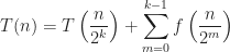
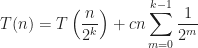


Assuming 


Implementation
In terms of parallelizing the sequential implementation, an addition interface, IThreadedListOperation was added to provide a BeginOperation, EndOperation asynchronous programming model found in the .net world. After looking around the Java world, I didn’t encounter a preferred idiom, so I went with what I knew.
As I mentioned in the sequential approach, the original data structures were going to be arrays which have a guarantee of providing thread safe reads, but not necessarily thread safe writes. To avoid the issue all together, I decided that the IListOperations should always return a new List<T> instance so that only one thread at a time would be reading or manipulating that memory. Since I knew my implementation would not be sharing IListOperations between threads, I decided not to gold plate the implementation with synchronization constructs. If in the future such ability were required, I would go back and modify the code accordingly.
For the parallel implementation I took advantage of the fact that method arguments are evaluated left-to-right [3] to save one some space, but if the specification ever changed, then it would be more appropriate to move the out the leftSort.execute() and rightSort.executeEnd() methods up a line to form a more explicit operation.
package com.wordpress.antimatroid;

import java.util.List;
import java.util.RandomAccess;

abstract public class IThreadedListOperation
    <T, L extends List<T> & RandomAccess>
    implements Runnable, IListOperation<T, L> {

	private Thread thread;

	public void executeBegin() {
		if(thread != null)
			throw new IllegalStateException();

		thread = new Thread(this);
		thread.start();
	}

	public L executeEnd() {
		if(thread == null)
			throw new IllegalStateException();

		try {
			thread.join();
		} catch (InterruptedException e) {

		}

		return getResult();
	}

	public L execute() {
		if(thread != null)
			throw new IllegalStateException();

		run();
		return getResult();
	}

	abstract protected L getResult();
}
package com.wordpress.antimatroid;

import java.util.List;
import java.util.RandomAccess;

public class MergeSortThreadedListOperation
    <T extends Comparable<T>, L extends List<T> & RandomAccess>
    extends IThreadedListOperation<T, L> {

	private final L a;
	private L b;

	private final int threshold;

	public MergeSortThreadedListOperation(L a) {
		this(a, 1024);
	}

	public MergeSortThreadedListOperation(L a, int threshold) {
		if(a == null)
			throw new IllegalArgumentException("a must be non-null.");

		if(threshold <= 0)
			throw new IllegalArgumentException("threshold must be greater than zero.");

		this.a = a;
		this.threshold = threshold;
	}

	@Override
	public void run() {
		if(a.size() <= 1) {
			b = a;
			return;
		}

		if(a.size() <= threshold) {
			MergeSortListOperation<T, L> mergeSort = new MergeSortListOperation<T, L>(a);
			b = mergeSort.execute();
			return;
		}

		CopyListOperation<T, L> leftPartition
                = new CopyListOperation<T, L>(a, (a.size() / 2) +  a.size() % 2, 0);
		MergeSortThreadedListOperation<T, L> leftSort
                = new MergeSortThreadedListOperation<T, L>(leftPartition.execute());

		CopyListOperation<T, L> rightPartition
                = new CopyListOperation<T, L>(a, (a.size() / 2), (a.size() / 2) +  a.size() % 2);
		MergeSortThreadedListOperation<T, L> rightSort
                = new MergeSortThreadedListOperation<T, L>(rightPartition.execute());

		rightSort.executeBegin();

		MergeListOperation<T, L> merge
                = new MergeListOperation<T, L>(leftSort.execute(), rightSort.executeEnd());

        b = merge.execute();
	}

	@Override
	protected L getResult() {
		return b;
	}
}
Run Time Analysis
Noting that the time complexity for the parallel approach is
The trial methodology used in the sequential run time analysis is used once again to produce the following plot. Note that it begins at 2048 instead of 1. This was done so that only the parallel implementation was considered and not the sequential implementation when the input size is 

As presented in the plot, the regressed linear model in logarithmic space yields a satisfactory theoretical curve whose relative error to the empirical curve diminishes to zero as the input size increases.
Threshold Selection
As a thought experiment, it makes sense that as the threshold approaches infinity, that there is no difference between the sequential implementation and parallel one. Likewise, as the threshold approaches one, then the number of threads being created becomes exceedingly large and as a result, places a higher cost on parallelizing the operation. Someplace in the middle ought to be an optimal threshold that yields better run time performance compared to the sequential implementation and a pure parallel implementation. So a fixed input size should produce a convex curve as a function of the threshold and hence have a global minimum.

Conducting a similar set of trials as the ones conducted under the analysis of the sequential run time give a fully parallel and sequential curve which to evaluate where the optimal threshold resides. As the plot depicts, as the threshold approaches one, there is an increase in the processing taking the form of a convex curve. As the threshold exceeds the input size, then the sequential approach dominates. By conducting a Paired T-Test against the means of the two curves at each input size, 1024 was determined to be the optimal threshold based on the hardware used to conduct the trials. As the input size grows, it is evident that for thresholds less than 1024, the sequential approach requires less time and afterwards, the parallel approach is favorable.
Conclusion
In comparing the sequential and parallel implementations it was observed that the specified parallel implementation produced as much as a 2.65 factor improvement over the specified sequential implementation for megabyte sized lists.

Larger sized lists exhibited a declining improvement factor. It is presumed that as the input size grows that the amount of memory being created is causing excessive paging and as a result increasing the total run time and consequently reducing the improvement factor. To get around this limitation, the algorithm would need to utilize an in-place approach and appropriate synchronization constructs put into place to guarantee thread safety.
From a theoretical point of view, the improvement factor is the ratio of the run time of the sequential implementation to the parallel implementation. Using the time complexities presented, 
Footnotes
[1] This design decision is discussed in §4.7 of the Java Language Specification (3rd Edition) on reifiable types.
[2] The only two java.util classes providing this guarantee are ArrayList and Vector. Both of which implement the interface RandomAccess which is intended indicate that the class provides the (near) constant reading and writing of elements.
[3] The left-to-right order of operations is specified by §15.7.4 of the Java Language Specification (3rd Edition). Also worth noting the specification recommends against the practice of relying on this convention however in §15.7:
… It is recommended that code not rely crucially on this specification. Code is usually clearer when each expression contains at most one side effect, as its outermost operation, and when code does not depend on exactly which exception arises as a consequence of the left-to-right evaluation of expressions.
Viderefit: A Fitness Tracking App for Android Tablets
Introduction
Earlier this year I talked a bit about how I wanted to do some Android development to broaden my skill set. A little after that post I finally joined the 21st century and got an Android smartphone. Over the course of the summer I recorded all of my hikes and bike rides using Google’s My Tracks app. With my season coming to a close, I began to think about what I could do with all this data that I’d collected and what kind of insights I could discover. As a result, I came up with Viderefit, a simple Android tablet app, that allows me to review my changes in my performance over time. In this post I’m going to go over the product design cycle that went into making this first phase of the app- from brain storming, requirements building, user interface design, development, and post-production. I’ll be finishing up with some thoughts on the next set of features I’ll be contemplating to make the app commercially viable on Google Play.
Goals
For the first phase of the project, I set out with a few simple goals that I wanted to focus on:
- Since I’d been focusing research projects lately, I wanted to return to my roots and focus a bit on user experience and interface design. As a result, I decided It was important to me that I create an intuitive to use and visually appealing user interface that utilized a number of appropriate and meaningful information visualization techniques.
- I’ve done a lot of C# and Haskell development lately, and I wanted to do something relatively new, so I decided that I would develop on Android and dust off my Java skills from my college days.
- I wanted a “quick win”, something that I knew that I could complete over the course of a couple weeks. As a result, I decided that I would spend two weeks planning the project starting in mid-September, followed by another two weeks of development wrapping up mid-October, and the remaining two weeks of October to put together this post for a November publication.
Brain Storming
In thinking about what exactly it was I was going to build I began to ask myself, what questions should I be asking myself. So, I opened up Word and began typing out a bullet point list of questions to understand where I was going with this project. First thing I began to think about was what exactly is physical fitness? What exactly is being measured over time to show improvement? What exactly is improvement? I had some ideas from my experience, but nothing formal, so like anyone else, I jumped Wikipedia and came across the following quotation on the topic’s page:
Physical fitness has been defined as a set of attributes or characteristics that people have or achieve that relates to the ability to perform physical activity. – Physical Activity and Health: A Report of the Surgeon General
Not being completely satisfied with this, I looked around a bit more and found several pages outlining five areas that constitute physical fitness: aerobic or cardiovascular endurance, body composition, muscular strength, muscular endurance and finally, flexibility. Having felt like some progress was made, I moved on to the next question pertaining to measurements. Researching each of the five areas yielded some insights in the types of tests and measurements being used to assess these abilities such as VO2 max, BMI, ROM, S&R and a whole slew of alphabet soup measurements that I unfortunately did not have access to nor were they obtainable from the available set of data.
Thinking a bit more about the data that was available to me, it was clear the only area of physical fitness I could focus on was aerobic endurance. Despite the fact I lacked sufficient data to derive some of the formal measures of physical fitness, I could derive some common sense measures to relate my performance over time. Am I going longer, going further, going faster as I got deeper into my season? Is my improvement uniform over time or did I hit any plateaus? And so on. To explore these ideas, I exported all of the My Tracks data from my smartphone to a SD Card and combined the results using a throwaway C# application and loaded the combined CSV file into Excel.
 |
Based on my explorations in Excel, I decided that I had the data I needed to answer the types of common sense question I was thinking about and decided what I was after was three different views of my data: a summary dashboard, performance reporting and a raw view of the data.
Requirements
In deciding on my requirements, I thought a bit about what I had read in Ben Fry‘s Visualizing Data: Exploring and Explaining Data, that exploring most data sets consists of acquiring, parsing, filtering, mining, representing, refining and interacting with the data set. Keeping that in mind, I decided that I would likely have a series of tabs providing different views of the underlying data and sets of tools on each tab to assist in that data’s interpretation.
The summary dashboard is about capturing the “big picture” of the underlying data. In thinking about what was important to me, I wanted to capture how far I’d gone, how long I’d spent and how many times I went out. Each of these three sections would be broken down into a total, a percentage of some reference figures (e.g., the distance between cities), a chart showing the total broken out by activity type and month, box plot showing the underling distribution, a stacked bar chart showing the underlying activity distribution and finally the longest, furthest, or most common track was to be presented.
Performance reporting is about enabling the end user to explore the underlying data. In essence, enabling the end user to chart different features plotted against one another and summarized according to some scheme. The user would then be able to filter by activity type and break the data set out into pre-season, mid-season and post-season components to better see trends taking place over time.
Finally, the raw view of the data provides a listing of all the tracks that were captured. Selecting a track displays a speed and altitude plot along with box plots for speed and altitude for the track in addition to box plots for the season so that the user can compare how a particular track compares to seasonal statistics.
Design
With an idea of the type of requirements that would be needed, it is time to flush out what the user interface will look like and how the user will interact with it. There are a lot of great products out there for mocking up user interfaces, I’ve used Balsamiq and really enjoyed it, but decided for this project, I would keep things simple and just mock things up in Photoshop since it’s easy to work with and low fidelity designs are all that’s needed at this point.
The summary dashboard incorporates the requirements into a vertical three panel design capturing distance, time and frequency of the underlying data. The dashboard is meant to be looked at and not interacted with, as a result the only thing the end user can do at this point is click on other tabs.
 |
Bulk of the features in the application will appear on the performance reporting tab. The user will be able to select x-Axis, y-Axis features and y-Axis feature aggregation strategy in order to plot out the results in the right-hand chart area. Beneath the selection criteria are checkboxes for splitting the data out in to full season, pre-season, mid-season and post-season components. Finally, the user can filter out different activities by checking each activity for exclusion or inclusion.
 |
The view of the raw data is to provide a view outlining all of the user’s tracks. Each track listing includes the name of the track, date, length, duration and a altitude sparkline. Clicking on a track reveals a speed and altitude plot along with the box plots described in the previous section.
 |
Development
Based on the planning done earlier in the project, development was a matter spending some time in IntelliJ, translating the design into the appropriate Android conventions and implementing the necessary logic to calculate various statistics and data calculations.
Much of what was needed to implement the application was available in the JDK and Android SDK, however there were a few areas I felt I could leverage existing open source libraries without having to roll my own solution (especially given the timeline I had decided upon):
- For charting I decided to use achartengine (1.0.0) since it looked to be the most stable and used charting library for Android.
- To parse the CSV file containing all of the track information, I went with opencsv (2.3) since it seems to most widely used. Although it does look like an Apache Commons CSV package is in the works but not yet final.
- Since the time and date handing in Java is embarrassingly lacking in JDK 1.6, I ended up using joda-time (2.1) for presenting end user friendly date and time representations.
The three libraries are all licensed under the Apache License 2.0
In terms of code organization and events that take place, the application is structured around Android’s fragment approach to deal with having to provide different views based on the device being used. Since the focus of the application was to develop a tablet application, no additional layouts were developed to support smaller screen sizes. The main activity consists of loading data from an SD card and creating handlers for tab events for each of the three tabs. Each individual tab consists of a replicated paradigm of master-detail fragments and additional settings that are passed between fragments as bundles whenever an end user event takes place.
 |
The referenced packages: common, controls, reporting and serialization contain classes for binding views to data, data aggregation (essentially a watered-down version of .NET’s LINQ and Haskell’s higher order functions), and classes for loading track data into memory.
Post-production
With development complete, I set out to do some polishing and make the application visually consistent. To start things off, I wanted to settle on a color palette for the application. This was done by sampling the HSB space on 60 degrees increments of hue offset by 0, 15, and 30 degrees of hue, with fixed 100% saturation and 80% brightness giving a vibrant 24 color palette to work with.
 |
Once the color scheme was established, it was a matter of going through the application and making sure each user interface element was using the correct color resource. Once the colors were applied, I focused on applying a consistent spacing between all of the UI elements- specifically 16 dp and 8 dp depending on the context and bordering between components. From there, each chart was examined to make sure that the axes units and labels were presented correctly. One gripe about achartengine is that I was unable to find a way to set the axis title’s padding, so there is some overlap between the axis value labels and the axis title.
With the application spruced up, it was on to icon design and selection. For the application icon I decided to to do a simple vector-based tri-folded map with an overlaid panel and chart.
For the icons to be used in the application, I used those found in Google’s My Tracks app since those icons are available under a Creative Commons 3.0 BY-SA license and represent the vast majority of data that would be imported. Worth noting that most of those icons are based on the National Park Service’s Map Symbols Collection. Future versions of Viderefit will likely switch over to the NPS set since they represent a more considerable collection of activities and the collection is under a public domain license.
Last thing to settle on was the name of the application. During development the name was simply “My Track Visualizer”, but I wanted the app to be more than that, so I decided on “SeeFit” or “cFit”, whichever happened to be available. After a Google search, neither were available so, I decided to use the Latin word for “to see”, Videre, and luckily “Viderefit” didn’t show up in any Google search results, so presumably nobody else has taken it.
End result
After finishing post-production, the application was looking much more consistent and polished. Below are screenshots of each tab taken from my 10.1″ Acer Iconia Tab A500 development device.
 |
 |

|
Future Work
In thinking about what it will take to get this product market worthy, there are a few things that stand out in my mind:
- Data importing – for this project the data resided on an external SD card and was loaded into memory from a parsed CSV file. Ideally, the end user should be able to import data from multiple applications and in varying formats such that the data is stored more efficiently using the built-in SQLite capabilities of the platform.
- Data exporting – one open question is how this application fits into the broader fitness application ecosystem and what exportable data is of use to other applications.
- Territory – the project omits any presentation of actual GPS data recorded during each session. For those individuals who are more interested in where they’ve been over their measurements, it seems a territory view would be a selling point. In addition, some form of integration done with the Google Maps API would also help visualize territory and speeds on the map over time.
- Additional screen support – right now the application was designed specifically for tablets, but other users may wish to use this application on their smartphone.
- Goal support – having reviewed other applications on the market, the idea of goal tracking is a recurring theme. To make the product more marketable, it would be useful to add in this kind of functionality.
Conclusion
Reflecting back on the goals I set out at the beginning of the project, I feel I made an intuitive and easy to use product consisting of appropriate information visualization techniques; worked on a new platform other than my typical C# and Haskell environments; finally, managed to complete the project according to the timeline I established by finishing all work a full two weeks sooner than originally scheduled. Working on a new platform and hardware was a fun experience. With the work that I’ve done, I feel that I can proceed onto the next phase of the project and determine how to get the application ready for the marketplace and hopefully bring in some revenue in the process.
Category Recognition of Golden and Silver Age Comic Book Covers
Introduction
Motivation
For a while now, I’ve been wanting to work on a computer vision project and decided for my next research focused project that I would learn some image processing and machine learning algorithms in order to build a system that would classify the visual contents of images, a category recognizer. Over the course of the summer I researched several techniques and built the system I had envisioned. The end result is by no means state of the art, but satisfactory for four months of on-and-off development and research. The following post includes my notes on the techniques and algorithms that were used in the project followed by a summary of the system and its performance against a comic book data set that was produced during development.
Subject Matter
The original subject matter of this project were paintings from the 1890s done in the Cloisonnism art style. Artists of the style are exemplified by Emile Bernard, Paul Gaugin and Paul Serusier. The style is characterized by large regions of flat colors outlined by dark lines; characteristics that would be easy to work with using established image processing techniques. During development, it became evident that no one approach would work well with these images. As an alternative, I decided to work with Golden and Silver Age comic book covers from the 1940s to 1960s which also typified this art style. Many of the comic books were drawn by the same individuals such as Jack Kirby, Joe Shuster and Bob Kane. As an added benefit, there are thousands of comic book covers available online compared to the dozens of Cloisonnism paintings.
Image Processing
Representation
An image is a function, 


|
Like any other vector field, transformations can be applied to the image to yield a new image, 
There are many different instances of these types of filters, but only those used in this project are discussed below. Computational complexity and efficient algorithms for each type of filter are also discussed where appropriate.
Point-based Filters
Point-based filters, 

Grayscale Projection
It is helpful to collapse the RGB channels of an image down to a single channel for the purpose of simplifying filter results. This can be done by using a filter of the form 

Thresholding
A threshold filter serves as a way to accentuate all values in the image greater than or equal to a threshold, 
The first variety is the step threshold filter, 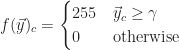
The second variety is a logistic threshold filter, 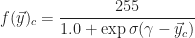

|
 ), logistic threshold filter (
 ), and logistic threshold filter (
 ).
). Neighbor-based Filters
All neighbor-based filters take the output vectors neighboring an input vector to calculate a new output vector value. How the neighboring output vectors should be aggregated together is given by a kernel image, 
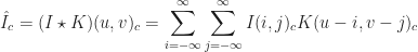
Neighbor-based filters can be applied naïvely in quartic time as a function of the image and kernel dimensions, 

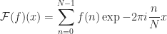
The Discrete Fourier Transform is a way of converting a signal residing in the spatial domain into a signal in the frequency domain by aggregating waveforms of varying frequencies where each waveform is amplified by its corresponding value in the input signal. The Inverse Discrete Fourier Transform maps a frequency domain signal back to the spatial domain.

Applying the Discrete Fourier Transform to a convolution, 

The improved time complexity is achieved by using a divide a conquer algorithm known as the Fast Fourier Transform which takes advantage of the Danielson-Lanczos Lemma which states that the Discrete Fourier Transform of a signal can be calculated by splitting the signal into two equal sized signals and computing their Discrete Fourier Transform.
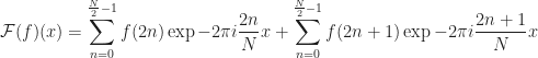


For the purposes of image processing, we use the two-dimensional Discrete and Inverse Discrete Fourier Transform.
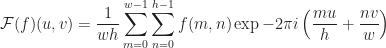
The expression can be rearranged to be the Discrete Fourier Transform of each column in the image and then computing the resulting Discrete Fourier Transform of those results to obtain the full two-dimensional Discrete Fourier Transform.
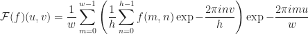
As a result, we can extend the Fast Fourier Transform in one dimension easily into two dimensions producing a much more efficient time complexity.
Weighted Means: Gaussian and Inverse Distance
Weighted mean filters are used to modify the morphology of an image by averaging neighboring output vectors together according to some scheme.
A Gaussian filter is used to blur an image by using the Gaussian distribution with standard deviation,
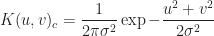
The inverse distance filter calculates how far the neighboring output vectors are with respect to the new output vector being calculated. Each result is also scaled by the parameter,

Laplacian
A Laplacian filter detects changes in an image and can be used for sharpening and edge detection. Much like in calculus of a single variable, the slope of a surface can be calculated by the Gradient operator, 

Since an image is a discrete function, the Laplacian operator needs to be approximated numerically using a central difference. 


|
 ), inverse distance filter (
 ) and Laplacian filter.
 Image-based Filters
Image-based filters calculate some information about the contents of the image and then use that information to generate the appropriate point-based and neighbor based filters.
Normalization
The normalization process computes the minimum, 


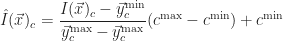
This particular image-based filter can be applied in quadratic time,

|
Edge Detection
Edge detection is the process of identifying changes (e.g., texture, color, luminance and so on) in an image. As alluded to in the image processing section, the Laplacian filter is central to detecting edges within an image. As a result A sequence of filters is used before and after a Laplacian filter to produce a detector that consistently segments comic book covers. The following sequence of filters was used.
- Grayscale Projection – Since all logical components of a comic book cover are separated by inked lines, it is permissible to ignore the full set of RGB channel information and collapse the image down to a grayscale image.
- Normalization – It is conceivable that the input image has poor contrast and brightness. To ensure that the full range of luminescence values are presented, the image is normalized.
- Gaussian (
) – An image may have some degree of noise superimposed on the image. To reduce the noise, the image is blurred using a Gaussian filter with a standard deviation of
. This is enough to smooth out the image without distorting finer image detail.
- Laplacian – Once the image has been prepared, its edges are calculated using the Laplacian filter.
- Normalization – Most of the changes in the image may be subtle and need to make sure that all edge information is accentuated as much as possible by applying a normalization filter.
- Step Threshold (
) – Since a partial edge isn’t particularly useful information, any edge RGB value less than
is attenuated to zero and all other values accentuated to
- Inverse Distance (
) – It is possible that during the threshold process that discontinuities were introduced into some of the edges. To mitigate this impact, an inverse distance filter is used to inflate existing edges and intensify the result with a gain of
 |
The complete edge detection process takes computational complexity of
Segmentation
With the edge image it is possible to segment the image into its visual components. This is achieved by doing a flood fill on the image and using the edge image as the boundaries for the fill. Once the fill runs out of points to flood, the segment is complete and the next remaining point in the image is considered. To reduce the number of minuscule segments, only those segments representing 

|
Machine Learning
Classifiers
The task of classification is to identify decision boundaries separating all of the classification within the data set. Such data sets can be linearly or non-linearly separable and as a result, classifiers were developed to solve the linear case and then adapted to deal with the more complicated non-linear case. While there are a number of classifiers, only the K-Nearest Neighbor and Support Vector Machine classifiers were researched and implemented in this project.
K-Nearest Neighbor
The K-Nearest Neighbor classifier is an online classifier which operates under the assumption that a yet to be classified vector is most likely to be the same classification as those 
Distance can be measured in a variety of ways for arbitrary vectors, 

The Manhattan distance, 


Two factors affect the efficacy of the algorithm. The first is the dimension of the data, 


|
Support Vector Machine
Formulation
The Support Vector Machine classifier is an offline linear, binary classifier which operates under the assumption that a training set, 


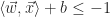


|
 .
.
The hyperplane is padded by two hyperplanes separated by an equal distance to the nearest training examples of each classification. The span between the supporting hyper planes is the margin. The goal then is to pick a hyperplane which provides the largest margin between the two separable classifications. The margin between the supporting hyperplanes is given by 

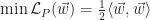

To find the optimal parameters, it is easier to translate the problem into a dual form by applying the technique of Lagrange Multipliers. The technique takes an objective function, 


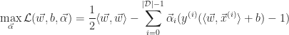


The next step is to differentiate the objective function with respect to the parameters to determine the optimal solution. Since the function is concave, the results will yield the desired maximum constraints.
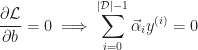
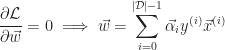
As a result the dual problem can be written as the following:
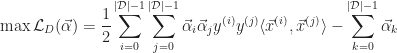
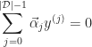
Handling of non-linearly separable data
In the event that the data is not linearly separable, then an additional parameter, 
Non-linear classification
By way of Mercer’s Theorem, the linear Support Vector Machine can be modified to allow for non-linear classification through the introduction of symmetric, positive semidefinite kernel functions, 


And the decision hyperplane function then becomes:
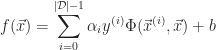
The following are some typical kernels:
- Linear –
- Polynomial –
- Radial basis function –
- Sigmoid –


From a practical point of view, only the linear and radial basis function kernels from this list should be considered since the polynomial kernel has too many parameters to optimize and the sigmoid kernel does not satisfy the positive semidefinite kernel matrix requirement of Mercer’s Theorem.
Algorithmic details
The Support Vector Machine classifier can be implemented using a quadratic programming solver or by incremental descent algorithms. Both methods work, but are difficult to implement and expensive to procure. An alternative is the Sequential Minimal Optimization algorithm developed by John Platt at Microsoft Research. The algorithm works by analytically solving the dual problem for the case of two training examples then iterating over all of the lagrange multipliers verifying that the constraints are satisfied. For those that are not, the algorithm computes new lagrange multiplier values. The full details of the algorithm can be found in Platt’s paper.
The time complexity of the algorithm is quadratic with respect to the number of training samples and support vectors
The time complexity of evaluating the decision function is linear with respect to the number of support vectors 
Multiclass Classification
The classification methods presented in the previous section are utilized as binary classifiers. These classifiers can be used to classify multiple classifications by employing a one-vs-all or all-vs-all approach. In the former a single classification is separated from the remaining classifications to produce
In the latter, a single classification is compared individually to each other classification resulting in 
Both methods have their place. The benefit of a one-vs-all approach is that there are fewer classifiers to maintain. However, training a single classifier on a complete data set is time consuming and can give deceptive performance measures. All-vs-all does result in more classifiers, but it also provides for faster training which can be easily parallelized on a single machine and distributed to machines on a network.
Classifier Evaluation
Individual classifiers are evaluated by training the classifier against a data set and then determining how many correct and incorrect classifications were produced. This evaluation produces a confusion matrix.
| Predicted Classification | ||||
|---|---|---|---|---|
| Positive | Negatives | Total | ||
| Actual Classification | Positive | (TP) True Positive | (FN) False Negative | (AP) Actual Positives |
| Negatives | (FP) False Positive | (TN) True Negative | (AN) Actual Negatives | |
| Total | (PP) Predicted Positives | (PN) Predicted Negatives | (N) Examples | |
The confusion matrix is used to calculate a number of values which are used to evaluate the performance of the classifier. The first of which is the accuracy and error of the classifier. Accuracy measures the number of instances where the actual and predicted classifications matched up and the error for when they do not.

Since we should expect to get different results each time we evaluate a classifier, the values that we obtain above are sample estimates of the true values that are expected. Given enough trails and measurements, it is possible to determine empirically what the true values actually are. However, this is time consuming and it is instead easier to use confidence intervals to determine what interval of values a measurement is mostly likely to fall into.
Training and Testing
Each of the classifiers presented have some number of parameters that must be determined. The parameters can be selected by having some prior knowledge or by exploring the parameter space and determining which parameters yield optimal performance. This is done by performing a simple grid search over the parameter space and evaluating and attempting to minimize the error.
K-folds cross-validation is used at each grid location to produce a reliable measure of the error. The idea is that a data set is split into 
System
Implementation
The system was implemented in C# 4.0 on top of the Microsoft .NET Framework. The user interface was written by hand using the WinForms library. No other third-party libraries or frameworks were used. When possible, all algorithms were parallelized to take advantage of multi-core capabilities to improve processing times.
Summary
The system consists of two modes of operation: training and production. In training, a human classifier labels image segments with an appropriate classification. New image segments are then taken into consideration during the training of machine learning algorithms. Those algorithms producing the lowest error for a given classification are then used in production mode. During production, a user submits an image and each image segment is then evaluated against the available classifiers. Those image segments are then presented to the user with the most likely classification. These two modes along with their workflows and components are illustrated in the following diagram.

|
Training Mode
Data Set Construction
The user interface of the system allows users to add an image segment to a local data set of images. Once added, the image is then processed to yield image segments. The user can then label an image segment by editing the segment and moving on to the next image segment. This allows for easy and efficient human classification of data. If the user does not wish to keep the image, he or she may remove the image from the data set as well.

|
Data Set Cleaning
During the construction phase, errors may be introduced into the data set typically in the case of typos or forgetting which segment was currently being edited. The data set is cleaned by listing out all available classifications and presenting the user with all available segments associated with that classification. The user can then review the image segment as it was identified in the source image. If the user does not wish to keep the classification, he or she may remove the image from the data set as well.

|
Data Set Statistics
The data set consists of 496 comic book covers pulled from the Cover Browser database of comic book covers. The first 62 consecutive published comic book covers where used from Action Comics, Amazing Spider-man, Batman, Captain America, Daredevil, Detective Comics, Superman, and Wonder Woman and then processed by the image processing subsystem yielding 24,369 image segments. 11,463 of these segments represented classifiable segments which were then labeled by hand over the course of two weeks; the remaining segments were then discarded.

|
In total, there were 239 classifications identified in the data set among 18 categories. Text, clothing, geography, and transportation categories accounting for 90% of the data set. Since the majority of classification were incidental, only those classifications having 50 or more image segments were considered by the application leaving a total of 38 classifications.
Classifier Evaluation
For the 38 classifications meeting the minimum criteria for classification, the K-Nearest Neighbor approach worked well in distinguishing between text classifications from other classifications and between intra-text classifications for both all-vs-all and one-vs-all schemes.

|

|
| All-vs-All K-Nearest Neighbor Performance. | One-vs-All K-Nearest Neighbor Performance. |
The Support Vector Machine approach presented unremarkable results for both all-vs-all and one-vs-all methods. In the former, only a few pairings resulted in acceptable error rates whereas the later presented only a couple acceptable error rates.

|

|
| All-vs-All Support Vector Machine Performance. | One-vs-All Support Vector Machine Performance. |
For both classification methods presented, the all-vs-all method yielded superior results to the one-vs-all method. In comparing the two classifier methods, the K-Nearest Neighbor seems to have done better than the Support Vector Machine approach, contrary to what was expected from literature. Both classifier methods are used in production mode.
Production Mode
Production mode allows the end user to add an image to the data set and then review the most likely classifications produced by evaluating each image segment against the available set of classifiers. The end user is then expected to review each segment and accept or reject the suggested classification. Aside from this additional functionality, production mode is nearly identical in functionality to training mode.

|
Conclusions
The time spent on this project was well spent. I met the objectives that I laid out at the beginning of the project and now have a better understanding of the image processing algorithms and machine learning concepts from a theoretical and practical point of view.
Future Work
Segmentation
One issue with the existing implementation is that it over segments the image. Ideally, fewer segments would be produced that are more closely aligned with their conceptual classification. There are a number of popular alternatives to the approach taken, such as level set methods, which should be further investigated.
Classification
The approach taken to map scaled versions of the image segments to a 
System User Interface
While it was disappointing to have spent so much time building a data set only to have to limit what was considered, it assisted me in building a user interface that had to be easy and fast to use. The application can certainly be developed further and adapted to allow for other data sets to be constructed, image segmentation methods to be added and additional classifications to be evaluated.
System Scalability
The system is limited now to a single machine, but to grow and handle more classifications, it would need to be modified to run on multiple machines, have a web-based user interface developed and a capable database to handle the massive amounts of data that would be required to support a data set on the scale of the complete Cover Browser’s or similar sites’ databases (e.g., 450,000 comic book covers scaled linearly would require 546 GiB of storage.) Not to mention data center considerations for overall system availability and scalability.
References
Aly, Mohamed. Survey on Multiclass Classification Methods. [pdf] Rep. Oct. 2011. Caltech. 24 Aug. 2012.
Asmar, Nakhle H. Partial Differential Equations: With Fourier Series and Boundary Value Problems. 2nd ed. Upper Saddle River, NJ: Pearson Prentice Hall, 2004. Print.
Bousquet, Olivier, Stephane Boucheron, and Gabor Lugosi. “Introduction to Statistical Learning Theory.” [pdf] Advanced Lectures on Machine Learning 2003,Advanced Lectures on Machine Learning: ML Summer Schools 2003, Canberra, Australia, February 2-14, 2003, Tübingen, Germany, August 4-16, 2003 (2004): 169-207. 7 July 2012.
Boyd, Stephen, and Lieven Vandenberghe. Convex Optimization [pdf]. N.p.: Cambridge UP, 2004. Web. 28 June 2012.
Burden, Richard L., and J. Douglas. Faires. Numerical Analysis. 8th ed. Belmont, CA: Thomson Brooks/Cole, 2005. Print.
Caruana, Rich, Nikos Karampatziakis, and Ainur Yessenalina. “An Empirical Evaluation of Supervised Learning in High Dimensions.” [pdf] ICML ’08 Proceedings of the 25th international conference on Machine learning (2008): 96-103. 2 May 2008. 6 June 2012.
Fukunaga, Keinosuke, and Patrenahalli M. Narendra. “A Branch and Bound Algorithm for Computing k-Nearest Neighbors.” [pdf] IEEE Transactions on Computers (1975): 750-53. 9 Jan. 2004. 27 Aug. 2012.
Gerlach, U. H. Linear Mathematics in Infinite Dimensions: Signals, Boundary Value Problems and Special Functions. Beta ed. 09 Dec. 2010. Web. 29 June 2012.
Glynn, Earl F. “Fourier Analysis and Image Processing.” [pdf] Lecture. Bioinformatics Weekly Seminar. 14 Feb. 2007. Web. 29 May 2012.
Gunn, Steve R. “Support Vector Machines for Classification and Regression” [pdf]. Working paper. 10 May 1998. University of Southampton. 6 June 2012.
Hlavac, Vaclav. “Fourier Transform, in 1D and in 2D.” [pdf] Lecture. Czech Technical University in Prague, 6 Mar. 2012. Web. 30 May 2012.
Hsu, Chih-Wei, Chih-Chung Chang, and Chih-Jen Lin. A Practical Guide to Support Vector Classification. [pdf] Tech. 18 May 2010. National Taiwan University. 6 June 2012.
Kibriya, Ashraf M. and Eibe Frank. “An empirical comparison of exact nearest neighbour algorithms.” [pdf] Proc 11th European Conference on Principles and Practice of Knowledge Discovery in Databases. (2007): 140-51. 27 Aug. 2012.
Marshall, A. D. “Vision Systems.” Vision Systems. Web. 29 May 2012.
Panigraphy, Rina. Nearest Neighbor Search using Kd-trees. [pdf] Tech. 4 Dec. 2006. Stanford University. 27 Aug. 2012.
Pantic, Maja. “Lecture 11-12: Evaluating Hypotheses.” [pdf] Imperial College London. 27 Aug. 2012.
Platt, John C. “Fast Training of Support Vector Machines Using Sequential Minimal Optimization.” [pdf] Advances in Kernel Methods – Support Vector Learning (1999): 185-208. Microsoft Research. Web. 29 June 2012.
Sonka, Milan, Vaclav Hlavac, and Roger Boyle. Image Processing, Analysis, and Machine Vision. 2nd ed. CL-Engineering, 1998. 21 Aug. 2000. Web. 29 May 2012.
Szeliski, Richard. Computer vision: Algorithms and applications. London: Springer, 2011. Print.
Tam, Pang-Ning, Michael Steinbach, and Vipin Kumar. “Classification: Basic Concepts, Decision Trees, and Model Evaluation.” [pdf] Introduction to Data Mining. Addison-Wesley, 2005. 145-205. 24 Aug. 2012.
Vajda, Steven. Mathematical programming. Mineola, NY: Dover Publications, 2009. Print.
Welling, Max. “Support Vector Machines“. [pdf] 27 Jan. 2005. University of Toronto. 28 June 2012
Weston, Jason. “Support Vector Machine (and Statistical Learning Theory) Tutorial.” [pdf] Columbia University, New York City. 7 Nov. 2007. 28 June 2012.
Zhang, Hui, Jason E. Fritts, and Sally A. Goldman. “Image Segmentation Evaluation: A Survey of Unsupervised Methods.” [pdf] Computer Vision and Image Understanding 110 (2008): 260-80. 24 Aug. 2012.
Copyright
Images in this post are used under §107(2) Limitations on exclusive rights: Fair use of Chapter 1: Subject Matter and Scope of Copyright of the of the Copyright Act of 1976 of Title 17 of the United States Code.
Summer
It’s time for my annual “It’s too beautiful outside to be inside” post. As next Fall begins to creep back onto my calendar, I’ll be wrapping up some projects that I’m currently working on and starting some new ones. Hoping to finish an Android tablet platformer, a computer vision project and a machine translation system by the end of the year. Smaller posts falling into the realm of algorithms, business and finance are also in the queue.
If you enjoy the content on this site, I recommend adding it to your RSS reader and keeping an eye out for future posts. In the mean time, take a look through the archives and find something interesting to read.
Tropical Representation of the All-Pairs Shortest Path Problem
Motivation
While I was doing my Abstract Algebra research the other month, I came across an interesting way of simplifying the representation of the all-pairs shortest path problem using Tropical Geometry. I thought it was pretty clever, so I thought I’d do a quick write-up.
Problem Statement
The all-pairs shortest path problem is to identify the minimum path cost, 


Proposition
Consider a weighted directed graph (digraph), 


Now, consider a semi-ring over 


Linear algebra constructs can be tropicalized to yield the familiar definitions for matrix addition and multiplication for matricies 


Given the two prior statements, the elegant solution to the all-pairs shortest path problem is given by taking powers of the adjacency matrix: 
Proof
To see how this works out, start with 


![\forall k \in [1, m]](https://s0.wp.com/latex.php?latex=%5Cforall+k+%5Cin+%5B1%2C+m%5D&bg=ffffff&fg=1c1c1c&s=0&c=20201002)
The result is a typical Bellman equation. A graph can have at most 

Example
As a worked example, consider the following graph whose set of vertices is given by the set 


The all-pairs shortest paths are given by the following calculations where the row and column coordinates correspond to the vertices of
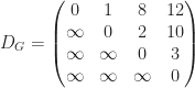
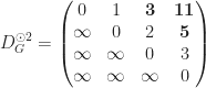

Computational Complexity
From asymptotic standpoint, tropical matrix multiplication is still on the order of traditional matrix multiplication of 


The time complexity can be further reduced to
References
“Floyd-Warshall’s Algorithm.” Algorithmist. Web. 12 Apr. 2012.
Cormen, Thomas H., Charles E. Leiserson, Ronald L. Rivest, and Clifford Stein. “25.2 The Floyd-Warshall Algorithm.” Introduction to Algorithms. 2nd ed. Cambridge, MA: MIT, 2001. 629-35. Print.
Diestel, Reinhard. Graph theory. Heidelberg New York: Springer, 2010.
Laface, Antonio. Introduction to Tropical Geometry [pdf]. 29 Nov. 2006. Web. 11 Apr. 2012.
Maclagan, Diane, and Bernd Sturmfels. Introduction to Tropical Geometry [pdf]. 4 Nov. 2009. Web. 9 Apr. 2012.
Mohri, Mehryar. “Semiring Frameworks and Algorithms for Shortest-Distance Problems” [pdf]. Journal of Automata, Languages and Combinatorics 7 (2002) 3: 321-50. 8 Aug. 2002. Web. 31 Mar. 2012.
Minesweeper Agent
Introduction

Lately I’ve been brushing up on probability, statistics and machine learning and thought I’d play around with writing a Minesweeper agent based solely on these fields. The following is an overview of the game’s mechanics, verification of an implementation, some different approaches to writing the agent and some thoughts on the efficacy of each approach.
Minesweeper
Background
Minesweeper was created by Curt Johnson in the late eighties and later ported to Windows by Robert Donner while at Microsoft. With the release of Windows 3.1 in 1992, the game became a staple of the operating system and has since found its way onto multiple platforms and spawned several variants. The game has been shown to be NP-Complete, but in practice, algorithms can be developed to solve a board in a reasonable amount of time for the most common board sizes.
Specification
Gameplay |
|
An agent,  , is presented a , is presented a  grid containing grid containing  uniformly distributed mines. The agent’s objective is to expose all the empty grid locations and none of the mines. Information about the mines’ grid locations is gained by exposing empty grid locations which will indicate how many mines exist within a unit (Chebyshev) distance of the grid location. If the exposed grid location is a mine, then the player loses the game. Otherwise, once all empty locations are exposed, the player wins. uniformly distributed mines. The agent’s objective is to expose all the empty grid locations and none of the mines. Information about the mines’ grid locations is gained by exposing empty grid locations which will indicate how many mines exist within a unit (Chebyshev) distance of the grid location. If the exposed grid location is a mine, then the player loses the game. Otherwise, once all empty locations are exposed, the player wins.
|
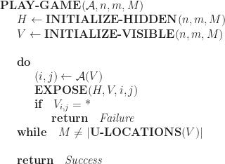
|
Initialization |
|
The board consists of hidden and visible states. To represent the hidden,  , and visible state, , of the board, two character matrices of dimension are used. , and visible state, , of the board, two character matrices of dimension are used.
Characters ‘0’-‘8’ represent the number of neighboring mines, character ‘U’ to represent an unexposed grid location and character ‘*’ for a mine. Neighbors of a grid location |

|
Exposing Cells |
|
|
The expose behavior can be thought of as a flood fill on the grid, exposing any empty region bordered by grid locations containing mine counts and the boundaries of the grid.
A matrix, If a cell location can be exposed, then each of its neighbors will be added to the stack to be inspected. Those neighbors that have already been inspected will be skipped. Once all the reachable grid locations have been inspected, the process terminates. |

|
 is the set of grid locations such that
  . By default,
  .
.

 , represents the topography of the board. A value of zero is reserved for sections of the board that have yet to be visited, a value of one for those that have, two for those that are boundaries and three for mines. A stack,
  , keeps track of locations that should be inspected.
 Verification
Methodology
Statistical tests are used to verify the random aspects of the game’s implementation. I will skip the verification of the game’s logic as it requires use of a number of different methods that are better suited for their own post.
There are two random aspects worth thinking about: the distribution of mines and the distribution of success (i.e., not clicking a mine) for random trials. In both scenarios it made since to conduct Pearson’s chi-squared test. Under this approach there are two hypotheses:
: The distribution of experimental data follows the theoretical distribution
: The distribution experimental data does not follow the theoretical distribution


Mine distribution
The first aspect to verify was that mines were being uniformly placed on the board. For a standard 


In the above experiment, 


Distribution of successful clicks
The second aspect to verify is that the number of random clicks before exposing a mine follows a hypergeometric distribution. The hypergeometric distribution is appropriate since we are sampling (exposing) without replacement (the grid location remains exposed after clicking). This hypothesis relies on a non-flood-fill exposure.
The distribution has four parameters. The first is the number of samples drawn (number of exposures), the second the number of successes in the sample (number of empty exposures), the third the number of successes in the population (empty grid locations) and the last the size of the population (grid locations): 
The expected frequencies for the hypergeometric distribution is given by 


In the above experiment 

Also included in the plot is the observed distribution for a flood based exposure. As one might expect, the observed frequency of more exposures decreases more rapidly than that of the non-flood based exposure.
Agents
Methodology
Much like how a human player would learn to play the game, I decided that each model would have knowledge of game’s mechanics and no prior experience with the game. An alternative class of agents would have prior experience with the game as the case would be in a human player who had studied other player’s strategies.
To evaluate the effectiveness of the models, each played against a series of randomly generated grids and their respective success rates were captured. Each game was played on a standard beginner’s ![[1, 10]](https://s0.wp.com/latex.php?latex=%5B1%2C+10%5D&bg=ffffff&fg=1c1c1c&s=0&c=20201002)
For those models that refer to a probability measure,
Marginal Model
DevelopmentThe first model to consider is the Marginal Model. It is designed to simulate the behavior of a naive player who believes that if he observes a mine at a grid location that the location should be avoid in future trials. The model treats the visible board,
|

|
 or (a)
  . This model picks the grid location with the greatest empirical probability of being empty:
Test Results
Since the mine distribution is uniform, the model should be equivalent to selecting locations at random. The expected result is that avoiding previously occupied grid locations is an ineffective strategy as the number of mines increases. This does however, provide an indication of what the success rate should look like for chance alone.

Conditional Model
DevelopmentOne improvement over the Marginal Model is to take into account the visual clues made visible when an empty grid location is exposed. Since an empty grid location represents the number of neighboring mines, the Conditional Model can look at these clues to determine whether or not an unexposed grid location contains a mine. This boils down to determining the probability of As in the case of the Marginal Model, the Conditional Model returns the grid location that it has determined has the greatest probability of being empty given its neighbors:
|
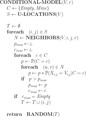
|
 . A simplification in calculating the probability is to assume that each piece of evidence is independent. Under this assumption the result is a
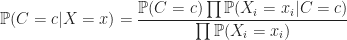
Test Results
The Naïve Bayes Classifier is regarded as being an effective approach to classifying situations for a number of different tasks. In this case, it doesn’t look like it is effective at classifying mines from non-mines. The results are only slightly better than the Marginal Model.

Graphical Model
DevelopmentOne shortfall of the Conditional Model is that it takes a greedy approach in determining which action to take. A more sophisticated approach is to not just consider the next action, but the possible sequence of actions that will minimize the possibility of exposing a mine. Each of the possible observable grids, It is possible to pick a path, Solving for
|
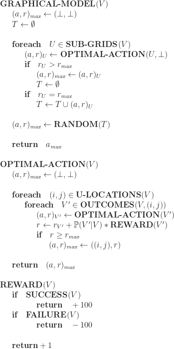
|
 , to the next observable state,
  . Each transition was achieved by performing an action,
  , on the state. The specific action,
  , is chosen from a subset of permitted actions given the state. Each transition has a probability,
  , of taking place.
 , through this graph that minimizes the risk by assigning a reward,
  , to each state and attempting to identify an optimal path,
  , from the present state that yields the greatest aggregate reward,

From the optimal walk, a sequence of optimal actions is determined by mapping
This description constitutes a Markov Decision Process. As is the case for most stochastic processes, it is assumed that the process holds the Markov Property; that future states only depend upon the current states and none of the prior states. In addition to being a Markov Decision Process, this is also an example of Reinforcement Learning.
First thing to observe is that the game state space is astronomical. For a standard beginner’s grid there is at most a sesvigintillion 
To simplify the state space, I chose to only consider 
Test Results
The Graphical Model produces results that are only a margin better than those of the Conditional Model.

Semi-deterministic Model
DevelopmentThe last model I’m going to talk about is a semi-deterministic model. It works by using the visible grid to infer the topology of the hidden grid and from the hidden grid, the topology that the visible grid can become. The grid can be viewed as a graph. Each grid location is a vertex and an edge is an unexposed grid location’s influence on another grid location’s neighbor mine count. For each of the exposed grid locations on the board, The model produces its inferred version, For each of the grid locations that are exposed and the inferred influence matches the visible count, then each of the neighbors about that location can be exposed provided they are not already exposed and not an inferred mine. From this set of possibilities, a mine location is chosen. When no mine locations can be determined, then an alternative model can be used. |

|
 , it’s neighbors,
  , are all mines when the number of inbound edges
  , matches the visible mine count
  .
. , of the influence graph
  by using the determined mine locations
 Test Results
Since the model is a more direct attempt at solving the board, its results are superior to the previously presented models. As the number of mines increases, it is more likely that it has to rely on a more probabilistic approach.

Summary
Each of the models evaluated offered incremental improvements over their predecessors. Randomly selecting locations to expose is on par with choosing a location based on previously observed mine locations. The Conditional Model and Graphical Model yield similar results since they both make decisions based on conditioned probabilities. The Semi-deterministic Model stands alone as the only one model that produced reliable results.

The success rate point improvement between the Condition and Marginal models is most notable for boards consisting of three mines and the improvement between Graphical and Semi-deterministic models for seven mines. Improvements between Random and Marginal models is negligible and between Conditional and Graphical is minor for all mine counts fewer than seven.

Given the mathematical complexity and nondeterministic nature of the machine learning approaches, (in addition the the complexity and time involved in implementing those approaches) they don’t seem justified when more deterministic and simpler approaches exist. In particular, it seems like most people have implemented their agents using heuristics and algorithms designed to solve constraint satisfaction problems. Nonetheless, this was a good refresher to some of the elementary aspects of probability, statistics and machine learning.
References
“Classification – Naïve Bayes.” Data Mining Algorithms in R. Wikibooks. 3 Nov. 2010. Web. 30 Oct. 2011.
“Windows Minesweeper.” MinesweeperWiki. 8 Sept. 2011. Web. 30 Oct. 2011.
Kaye, Richard. “Minesweeper Is NP-complete.” [pdf] Mathematical Intelligencer 22.2 (2000): 9-15. Web. 30 Oct. 2011.
Nakov, Preslav, and Zile Wei. “MINESWEEPER, #MINESWEEPER.” 14 May 2003. Web. 14 Apr. 2012.
Richard, Sutton, and Andrew G. Barto. “3.6 Markov Decision Processes.” Reinforcement Learning: An Introduction. Cambridge, Massachusetts: Bradford Book, 1998. 4 Jan. 2005. Web. 30 Oct. 2011.
Rish, Irene “An Empirical Study of the Naive Bayes Classifer.” [pdf] IJCAI-01 Workshop on Empirical Methods in AI (2001). Web. 30 Oct. 2011.
Russell, Stuart J., and Peter Norvig. Artificial Intelligence: A Modern Approach. Upper Saddle River, NJ: Prentice Hall/PearsonEducation., 2003. Print.
Sun, Yijun, and Jian Li. “Adaptive Learning Approach to Landmine Detection.” [pdf] IEEE Transactions of Aerospace and Electronic Systems 41.3 (2005): 1-9. 10 Jan. 2006. Web. 30 Oct. 2011.
Taylor, John R. An introduction to error analysis: the study of uncertainties in physical measurements. Sausalito, CA: University Science Books, 1997. Print.
