AWS | Antimatroid, The

Posts Tagged ‘AWS’

Distributed k-Means Clustering

Introduction

The applications of k-Means clustering are numerous in business, engineering, and science where demands for prompt insights and support for increasingly large volumes of data motivate the need for a distributed system that exploits the inherent parallelism of the algorithm on today’s emerging hardware accelerators (e.g., FPGA [3], GPU [15], many integrated core, multi-core [9]).

There are however a number questions that arise when building such a system: what accelerators should be supported, how to partition data in an unbiased way, how to distribute those partitions, what each participant will calculate from their partition, how those individual results will be aggregated, and finally, how to synchronize tasks between participants to complete the job as a whole.

Two of these questions will be the focus of this work: how to efficiently transfer data to workers, and how to synchronize them in the presence of transient workers. For the former, remote direct memory access (RDMA) is used to distribute disk-based data from a coordinator to workers, and an extension to synchronization barriers is developed to allow workers to leave ongoing calculations, and return without interrupting other workers.

How well the system solves these issues will be measured by observed transfer rates and per iteration synchronization times. To understand the system’s scalability and place in the broader distributed machine learning landscape, its runtime performance will be evaluated against Apache Spark. Based on these results, future work will be discussed on how to move forward with the study to create a system that can meet the ever growing demands of users.

Background

$1: \textbf{procedure } \textsc{k-Means}(C, X, d, N, K) \newline 2: \qquad \textbf{while } \text{not convered } \textbf{do } \newline 3: \qquad \qquad S_k \gets \{ x : k = \text{argmin}_{i} \lVert c_i - x \rVert_2, x \in X \} \newline 4: \qquad \qquad \Sigma_{k} \gets \sum_{x \in S_k} x \newline 5: \qquad \qquad \kappa_{k} \gets \lVert S_k \rVert \newline 6: \qquad \qquad c_{k} = \Sigma_{k} / \kappa_{k} \newline 7: \qquad \textbf{end while} \newline 8: \qquad \textbf{return } C \newline 9: \textbf{end procedure}$

k-Means clustering belongs to the family of expectation-maximization algorithms where starting from an initial guess $C$ , $K$ centroids are iteratively inferred from a dataset $X$ containing $N$ $\mathbb{R}^d$ vectors. Each iteration the partial sum $\Sigma_k$ , and quantity $\kappa_k$ of vectors nearest the $k^{th}$ centroid are aggregated. From these quantities the updated centroids $c_k$ can be calculated for the next iteration until the difference in magnitude from the former is less than some tolerance $\epsilon$ or a maximum number of iterations $I$ is observed providing a $\mathcal{O}(dIKN)$ linear time algorithm.

Parallelism is based on each participant $p$ being assigned a partition of the data so that instead of computing $\Sigma_k$ and $\kappa_k$ on the entirety of $X$ , it is on some disjoint subset $X_p$ s.t. $X = \cup_p X_p$ and $\cap_p X_p = \emptyset$ . When each participant has computed their $(\Sigma_k^p, \kappa_k^p)$ , pairs the resulting set of values can be aggregated $(\Sigma_k, \kappa_k) = \sum_{p} (\Sigma_k^p, \kappa_k^p)$ to yield the updated centroid values $c_k$ for the next iteration.

To ensure that participants can formulate a unified view of the data, it is assumed that user supplied datasets are adequately shuffled. If the natural clusters of the data were organized in a biased way, participants would individually draw different conclusions about the centroids leading to divergence. Further, it will be assumed that a loss of an unbiased partition will not degrade the quality of results beyond an acceptable threshold under certain conditions (cf. [6] for a rich formalism based on coresets to support this assumption).

RDMA

One of the failings of conventional network programming is the need to copy memory between user and kernel space buffers to transmit data. This is an unnecessary tax that software solutions shouldn’t have to pay with runtime. The high performance computing community addressed this issue with remote direct memory access [12] whereby specialized network hardware directly reads from, and writes to pinned user space memory on the systems. These zero-copy transfers free the CPU to focus on core domain calculations and reduces the latency of exchanging information between systems over 56 Gbps InfiniBand or 40 Gbps RoCE.

Barriers

Synchronization barriers allow a number of participants to rendezvous at an execution point before proceeding as a group (cf. [12] for a survey of advanced shared-memory techniques). Multi-core kernels in the system use a counting (centralized) barrier: the first $n-1$ threads that approach the barrier will enter a critical section, decrement a counter, and sleep on a condition variable; the last thread to enter the critical section will reset the counter and signal the condition variable to wake the other threads before leaving the critical section. At this point all threads are synchronized and can proceed as a group.

Since the emphasis of this work is on fault tolerance, distributed all-to-all and one-to-all message passing versions of the counting barriers are considered (cf. [4] for more advanced distributed methods). In the former, every participant will notify and wait to hear from every other participant before proceeding. In the latter, every participant will notify and wait to hear from a coordinator before proceeding. The all-to-all design most closely resembles a counting barrier on each participant, whereas the all-to-one resembles a counting barrier on a single participant.

Design

System participants consist of a single coordinator and multiple workers. A coordinator has the same responsibilities as a worker, but is also responsible for initiating a task and coordinating recovery. Workers are responsible for processing a task and exchanging notifications. A task is a collection of algorithm parameters (maximum iteration, convergence tolerance, number of clusters $K$ ), initial guesses ( $K$ by $d$ -dimensions), and unbiased partition of the dataset ( $N$ by $d$ -dimensions) that a participant is responsible for computing. Notifications consist of identifying information (host name, port), the current iteration, and partial results ( $K$ counts and $K$ by $d$ -dimensional sums).

Dataset Transfer

Figure 1: Example of transferring data between hosts using Accelio RDMA.

The first responsibility of the coordinator is to schedule portions of the disk based dataset to each worker. The coordinator will consult a list of participants and verify that the system can load the contents of the dataset into its collective memory. If so, the coordinator schedules work uniformly on each machine in the form of a task. A more sophisticated technique could be used, but a uniform loading will minimize how long each worker will wait on the others each iteration (assuming worker’s computing abilities are indistinguishable). The coordinator will sequentially distribute these tasks using RDMA, whereby the serialized contents of the task are read from disk into the coordinator’s user space memory are directly transfered over to an equally sized buffer in the worker’s user space memory before continuing on to the next worker.

Open source BSD licensed Accelio library [11] is used to coordinate the transfer of user space memory between machines as shown in Fig. (1). Following the nomenclature of the library, a client will allocate and register a block of user space memory; registration ensures that the operating system will not page out the memory while the network interface card is reading its contents. Next, the client will send a request asking the server to allocate an equally sized buffer. When the server receives this request, it will attempt to allocate and register the requested buffer. Once done, it will issue the rkey of the memory back to the client. An rkey is a unique identifier representing the location of the memory on the remote machine. Upon receipt of this information, the client will then ask the library to issue a RDMA write given the client’s and server’s rkeys. Since RDMA will bypass the server’s CPU all together, the server will not know when the operation completes; however, when the RDMA write completes, the client is notified and it can then notify the server that the operation is complete by terminating the connection and session.

During development it was discovered that the amount of memory that can be transfered this way is limited to just 64 MiB before the library errs out (xio_connection send queue overflow). To work around this limitation for larger partitions, the client will send chunks of memory in 64 MiB blocks. The same procedure detailed above is followed, however it is done for each block of memory with rkeys being exchanged for the appropriate offset on each client RDMA write complete notification until the entire contents of memory have been transfered. On each side the appropriate unregistering and deallocation of ancillary memory takes place and the worker deserializes the memory into a task before proceeding on to the first iteration of k-Means algorithm.

As an alternative to using direct RDMA writes, a design based on Accelio messaging was considered. In this design the client allocates memory for the serialized task and issues an allocation request to the server. The server services the request and the contents of memory are transfered in 8 KiB blocks before the exchange of messages is no longer necessary. While this approach requires fewer Accelio API calls to coordinate, it is significantly slower than the more involved direct RDMA based approach.

Iteration and aggregation

The k-Means algorithm is implemented as both a sequential and parallel multi-core kernel that can be selected at compile time. The sequential version is identical to what was discussed in the background, whereas the parallel kernel is a simplified version of the distributed system less data transfer and fault-tolerance enhancements. Data is partitioned onto threads equaling the total number of cores on the system. Each iteration threads are created to run the sequential kernel on each thread’s partition of the data. Once all the threads complete, they are joined back to the main thread where their partial results are aggregated by the main thread and used for the distributed synchronization.

Synchronization

In this distributed setting, the barrier must be able to accommodate the fluctuating presence of workers due to failures. Multiple designs were considered, but the all-to-all paradigm was chosen for its redundancy, local view of synchronization, and allows the coordinator to fail. The scheme may not scale well and future work would need to investigate alternative methods. Unlike the data transfer section, plain TCP sockets are used since the quantities of data being shared are significantly smaller.

A few assumptions need to be stated before explaining the protocol. First, the coordinator is allowed to be a single point of failure for recovery and failures for all participants are assumed to be network oriented up to network partitioning. Network partitions can operate independently, but cannot be reunified into a single partition. All other hardware resources are assumed to be reliable. Finally, the partition associated with a lost worker is not reassigned to another worker. It is simply dropped from the computations under the assumption that losing that partition will not significantly deteriorate the quality of the results up to some tolerance as mentioned in the introduction.

The first step to supporting transient workers is to support process restart. When a worker receives a task from the coordinator, it will serialize a snapshot to disk, service the task, and then remove the snapshot. When a worker process is started, it will deserialize an existing snapshot, and verify that the task is ongoing with the coordinator before joining, or discard the stale snapshot before awaiting the next task from the coordinator.

Figure 2: Example in which a worker reintegrates with the group after being offline for several iterations. Red lines denote blocking. (Timeout queries not shown.)

The distributed barrier next maintains a list of active, inactive and recovered participants in the system. The first phase of synchronization is the notification phase in which each participant will issue identifying information, current iteration, and its partial results for the k-Means algorithm to all other active participants. Those participants that cannot be reached are moved from the active to inactive list.

The second phase is the waiting phase in which a listening thread accumulates notifications on two separate blocking unbounded queues in the background. The recovery queue is for notifications, and the results queue for sharing partial results. For each active participant the results queue will be dequeued, and for each inactive participant, the results queue will be peeked and dequeued if nonempty. Because the results queue is blocking, a timeout is used to allow a participant to verify that another participant hasn’t gone offline in the time it took the participant to notify the other and wait for its response. If the other participant has gone offline, then it is moved from the active to inactive list, otherwise the participant will continue to wait on the other.

Each partial result from the results queue will be placed into a solicited or unsolicited list based on if its origin is a participant that was previously notified. The coordinator will then locally examine the unsolicited list and place those zero iteration requests in the recovered list when it is in a nonzero iteration. Workers will examine the unsolicited list and discard any requests whose iteration does not match their own.

The recovery phase begins by an inactive worker coming back online and sending their results to the coordinator, and then waiting to receive the coordinators results and a current iteration notification. The next iteration, the coordinator will look at its recovered list and send the current iteration to the recovering worker, then wait until it receives a resynchronized notification. Upon receiving the current iteration notification, the recovering worker will then go and notify all the other workers in the cluster of its results, and wait for them to response before issuing a resynchronized notification to the coordinator. At which point the recovering worker is fully synchronized with the rest of the system. Once the coordinator receives this notification on its recovery queue, it will move the recovering worker off the inactive and recovery lists and on to the active list before notifying the other workers of its results.

Once the notification and waiting phase have completed, all participants are synchronized and may independently find the next set of centroids by aggregating their partial results from both solicited and unsolicited lists, and then begin the next iteration of the k-Means algorithm. This process will continue until convergence, or the maximum number of iterations has been reached.

Experiments

Experiments were conducted on four virtual machines running Red Hat 4.8 with 8 GiB of RAM and single tri-core Intel Xeon E312xx class 2.6 GHz processor. Host machines are equipped with Mellanox Connect X-3 Pro EN network interface cards supporting 40 Gbs RoCE. Reported times are wall time as measured by gettimeofday. All C++98 source code compiled using g++ without any optimization flags.

Spark runtime comparison ran on Amazon Web Services Elastic Map Reduce with four m1.large instances running dual core Xeon E5 2.0 GHz processor with 7.5 GiB of RAM supporting 10 Gbps Ethernet. Spark 1.5.2 comparison based on MLlib KMeans.train and reported time measured by System.currentTimeMillis. All Java 1.7 code compiled by javac and packaged by Maven.

Transfer Rates

Figure 3: Transfer rates for variable block sizes up to 64 MiB and fixed 128 MiB payload.

Figure 4: Transfer rates for fixed 64 MiB RDMA and 8 KiB message based block sizes and variable payloads up to 7 GiB.

Fig. (3) shows the influence of block size on transfer rate of a fixed payload for RDMA based transfers. As mentioned in the design section, Accelio only supports block sizes up to 64 MiB for RDMA transfers. When the block size is 8 KiB, it takes 117x longer to transfer the same payload than when a block size of 64 MiB is used. This performance is attributed to having to exchange fewer messages for the same volume of data. For the payload of 128 MiB considered, a peak transfer rate of 4.7 Gbps was obtained.

Fig. (4) looks at the relationship of a fixed 64 MiB block size for RDMA transfers up to 7 GiB before exhausting available system resources. A peak transfer rate of 7.7 Gbps is observed which is still significantly less than the 40 Gbps capacity of the network. This would suggest a few possibilities: the Mellanox X-3 hardware was configured incorrectly, there may be network switches limiting the transfer of data, or that there is still room for improvement in the Accelio library.

It is unclear why there should be a kink in performance at 2 GiB. Possible explanations considered the impacts of hardware virtualization, influence of memory distribution on the physical DRAM, and potential Accelio issues. Further experiments are needed to pinpoint the root cause.

To demonstrate the advanced performance of Accelio RDMA based transfers over Accelio messaging based transfers, Fig. (4) includes transfer performance based on 8 KiB messaging. For the values considered, the message based approach was 5.5x slower than the RDMA based approach. These results are a consequence of the number of messages being exchanged for the smaller block size and the overhead of using Accelio.

Recovery time

Figure 5: Example of Worker A going offline at iteration 29 and coming back online at iteration 69.

Fig. (5) demonstrates a four node system in which one worker departs and returns to the system forty iterations later. Of note is the seamless departure and reintegration into the system without inducing increased synchronization times for the other participants. For the four node system, average synchronization time was 16 ms. For recovering workers, average reintegrate time was 225 ms with high variance.

Runtime performance

Table 1: Time in milliseconds spent in each task for 100 iterations, $d = 2, K = 4, N = 10,000,000$ .
	Total	Percentage
Sharing	721.9	6.7
Computing	8558.7	79.1
Synchronizing	1542.5	14.2
Unaccounted	6.2	0.1
Total	10820.4	100

Looking at the distribution of work, roughly 80% of the work is going towards actual computation that we care about and the remaining 20% what amounts to distributed system bookkeeping. Of that 20% the largest chunk is synchronization suggesting that a more efficient implementation is needed and that it may be worth abandoning sockets in favor of low latency, RDMA based transfers.

Figure 6: Runtime for varying input based Accelio messaging and sequential kernel, and RDMA and parallel kernel. The latter typically being 2.5x faster

Figure 7: Sequential, parallel, distributed versions of k-Means for varying input sizes with Spark runtime for reference.

Runtime of the system for varying inputs is shown in Fig. (6) based on its original Accelio messaging with sequential calculations, and final RDMA transfers with parallel calculations. The latter cuts runtime by 2.5x which isn’t terrible since each machine only has three cores.

The general runtime for different configurations for the final system is shown in Fig. (7). The sequential algorithm is well suited to process inputs less than ten thousand, parallel less than one million, and the distributed system for anything larger. In general, the system performed 40-50x faster than Spark on varying input sizes for a 9 core vs 8 core configuration. These are conservative estimates since the system does 100 fixed iterations, whereas and Spark’s MLlib $\text{k-Means} \lvert \lvert$ implementation stops as soon as possible (typically 5-10 iterations).

Figure 8: Speedup of the system relative to the sequential algorithm.

The overall speedup of the system relative to the sequential algorithm is shown in Fig. (8). For a 12 core system we observe at most a 7.3x runtime improvement (consistent with the performance and sequential vs. parallel breakdowns). In general, in the time it takes the distributed system to process 100 million entries, the sequential algorithm would only be able to process 13.7 million entries. Further optimization is desired.

Discussion

Related Work

The established trend in distributed machine learning systems is to use general purpose platforms such as Google’s MapReduce and Apache’s Spark and Mahout. Low latency, distributed shared memory systems such as FaRM and Grappa are gaining traction as ways to provide better performance thanks to declining memory prices and greater RDMA adoption. The next phase of this procession is exemplified by GPUNet [7], representing systems built around GPUDirect RDMA, and will likely become the leading choice for enterprise customers seeking performance given the rise of deep learning applications on the GPU.

The design of this system is influenced by these trends with the overall parallelization of the k-Means algorithm resembling the map-reduce paradigm and RDMA transfers used here reflecting the trend of using HPC scale technologies in the data center. Given that this system was written in a lower level-language and specialized for the task, it isn’t surprising that it delivered better performance (40-50x) than the leading general purpose system (Apache Spark) written in higher level language.

That said, given the prominence of general purpose distributed machine learning systems, specialized systems for k-Means clustering are uncommon and typically designed for unique environments (e.g., wireless sensor networks [13]). In the cases where k-means is investigated, the focus is on approximation techniques that are statistically bounded [6], and efficient communication patterns [2]; both of these considerations could further be incorporated into this work to realize better performance.

For the barrier, most of the literature focuses on static lists of participants in shared [12] and distributed [4] multi-processor systems with an emphasis on designing solutions for specific networks (e.g., n-dimensional meshes, wormhole-routed networks, etc). For barriers that accommodate transient participants, the focus is on formal verification with [8] and [1] focused on shared and distributed systems respectively. No performance benchmarks could be found for a direct comparison to this work, however, [5] presents a RDMA over InfiniBand based dissemination barrier that is significantly faster ( $\mu s$ vs $ms$ ) suggesting opportunities for future RDMA use.

Future Work

RDMA

Accelio provides a convenient API for orchestrating RDMA reads and writes at the expense of performance. Accelio serves a niche market and its maturity reflects that reality. There are opportunities to make Accelio more robust and capable for transferring large chunks of data. If this avenue of development is not fruitful, alternative libraries such as IBVerbs may be used in an attempt to obtain advertised transfer rates for RDMA enabled hardware.

As implemented, the distribution of tasks over RDMA is linear. This was done to take advantage of sequential read speeds from disk, but it may not scale well for larger clusters. Additional work could be done to look at pull based architectures where participants perform RDMA reads to obtain their tasks rather than the existing push based architecture built around RDMA writes. As well as exploring these paradigms for distributed file systems to accommodate larger datasets.

Calculations presented were multi-core oriented, but k-Means clustering can be done on the GPU as well. Technologies such as NVIDIA’s GPUDirect RDMA and AMD’s DirectGMA present an opportunity to accelerate calculations by minimizing expensive memory transfers between host and device in favor of between devices alone. Provided adequate hardware resources, this could deliver several orders magnitude faster runtime performance.

Kernel

As demonstrated in the experiments section, overall runtime is heavily dominated by the actual k-Means iteration suggesting refinements in the implementation will lead to appreciable performance gains. To this effect, additional work could be put into the sequential kernel to make better use of SIMD features of the underlying processor. Alternatively, the OpenBLAS library could be used to streamline the many linear algebra calculations since they already provides highly optimized SIMD features. Accelerators like GPUs, FPGAs, and MICs could be investigated to serve as alternative kernels for future iterations of the system.

Barrier

The barrier is by no means perfect and it leaves much to be desired. Beginning with allowing recovery of a failed coordinator, allowing reunion of network partitions, dynamic worker onboarding, and suspending calculations when too much of the system goes offline to ensure quality results. Once these enhancements are incorporated in to the system, work can be done to integrate the underlying protocols away from a socket based paradigm to that of RDMA. In addition, formal verification of the protocol would guide its use into production and on to larger clusters. The system works reasonably well on a small cluster, but further work is needed to harden it for modern enterprise clusters.

Overall System

As alluded to in the background, shuffling of data could be added to the system so that end users do not have to do so beforehand. Similarly, more sophisticated scheduling routines could be investigated to ensure an even distribution of work on a system of machines with varying capabilities.

While the k-Means algorithm served as a piloting example, work could be done to further specialize the system to accommodate a class of unsupervised clustering algorithms that fit the general map-reduce paradigm. The end goal is to provide a plug-n-play system with a robust assortment of optimized routines that do not require expensive engineers to setup, exploit, and maintain as is the case for most existing platforms.

Alternatively, the future of the system could follow the evolution of other systems favoring a generalized framework that enable engineers to quickly distribute arbitrary algorithms. To set this system apart from others, the emphasis would be on providing an accelerator agnostic environment where user specified programs run on whatever accelerators (FPGA, GPU, MIC, multi-core, etc.) are present without having to write code specifically for those accelerators. Thus saving time and resources for enterprise customers. Examples of this paradigm are given by such libraries as CUDAfy.NET and Aparapi for translating C# and Java code to run on arbitrary GPUs.

Conclusion

This work described a cross-platform, fault-tolerant distributed system that leverages the open source library Accelio to move large volumes of data via RDMA. Transfer rates up to 7.7 Gbps out of the desired 40 Gbps were observed and it is assumed if flaws in the library were improved, that faster rates could be achieved. A synchronization protocol was discussed that supports transient workers in the coordinated calculation of k-Means centroids. The protocol works well for small clusters, offering 225 ms reintegration times without significantly affecting other participants in the system. Further work is warranted to harden the protocol for production use. Given the hardware resources available the distributed system was 7.3x out of the desired 12x faster than the sequential alternative. Compared to equivalent data loads, the system demonstrated 40-50x better runtime performance than Spark MLlib’s implementation of the algorithm suggesting the system is a competitive alternative for k-Means clustering.

References

[1] Shivali Agarwal, Saurabh Joshi, and Rudrapatna K Shyamasundar. Distributed generalized dynamic barrier synchronization. In Distributed Computing and Networking, pages 143-154. Springer, 2011.

[2] Maria-Florina F Balcan, Steven Ehrlich, and Yingyu Liang. Distributed k-means and k-median clustering on general topologies. In Advances in Neural Information Processing Systems, pages 1995-2003, 2013.

[3] Mike Estlick, Miriam Leeser, James Theiler, and John J Szymanski. Algorithmic transformations in the implementation of k-means clustering on recongurable hardware. In Proceedings of the 2001 ACM/SIGDA ninth international symposium on Field programmable gate arrays, pages 103-110. ACM, 2001.

[4] Torsten Hoeer, Torsten Mehlan, Frank Mietke, and Wolfgang Rehm. A survey of barrier algorithms for coarse grained supercomputers. 2004.

[5] Torsten Hoeer, Torsten Mehlan, Frank Mietke, and Wolfgang Rehm. Fast barrier synchronization for inniband/spl trade. In Parallel and Distributed Processing Symposium, 2006. IPDPS 2006. 20th International, pages 7-pp. IEEE, 2006.

[6] Ruoming Jin, Anjan Goswami, and Gagan Agrawal. Fast and exact out-of-core and distributed k-means clustering. Knowledge and Information Systems, 10(1):17-40, 2006.

[7] Sangman Kim, Seonggu Huh, Yige Hu, Xinya Zhang, Amir Wated, Emmett Witchel, and Mark Silberstein. Gpunet: Networking abstractions for gpu programs. In Proceedings of the International Conference on Operating Systems Design and Implementation, pages 6-8, 2014.

[8] Duy-Khanh Le, Wei-Ngan Chin, and Yong-Meng Teo. Verication of static and dynamic barrier synchronization using bounded permissions. In Formal Methods and Software Engineering, pages 231-248. Springer, 2013.

[9] Xiaobo Li and Zhixi Fang. Parallel clustering algorithms. Parallel Computing, 11(3):275-290, 1989.

[10] Stuart P Lloyd. Least squares quantization in pcm. Information Theory, IEEE Transactions on, 28(2):129-137, 1982.

[11] Mellanox Technologies Ltd. Accelio – the open source i/o, message, and rpc acceleration library.

[12] John M Mellor-Crummey and Michael L Scott. Algorithms for scalable synchronization on shared-memory multiprocessors. ACM Transactions on Computer Systems (TOCS), 9(1):21-65, 1991.

[13] Gabriele Oliva, Roberto Setola, and Christoforos N Hadjicostis. Distributed k-means algorithm. arXiv, 2013.

[14] Renato Recio, Bernard Metzler, Paul Culley, Je Hilland, and Dave Garcia. A remote direct memory access protocol specication. Technical report, 2007.

[15] Mario Zechner and Michael Granitzer. Accelerating k-means on the graphics processor via cuda. In Intensive Applications and Services, 2009. INTENSIVE’09. First International Conference on, pages 7-15. IEEE, 2009.

Written by lewellen

2015-12-22 at 1:43 pm

Posted in Software Engineering

Tagged with Accelio, Amazon Web Services, AWS, Barrier, C++, Distributed Systems, Elastic Map Reduce, EMR, Fault-tolerance, Grad School, k-Means Clustering, RDMA, Remote Direct Memory Access

Large-Scale Detection and Tracking of Aircraft from Satellite Images

Introduction

Motivation

Historically, search and rescue operations have relied on on-site volunteers to expedite the recovery of missing aircraft. However, on-site volunteers are not always an option when the search area is very broad, or difficult to access or traverse as was the case when Malaysia Airlines Flight 370 disappeared over the Indian Ocean in March, 2014. Crowd-sourcing services such as tomnod.com have stepped up to the challenge by offering volunteers to manually inspect satellite images for missing aircraft in an attempt to expedite the recovery process. This process is effective, but slow. Given the urgency of these events, an automated image processing solution is needed.

Prior Work

The idea of detecting and tracking objects from satellite images is not new. There is plenty of academic literature on detection or tracking, but often not both for things like oil tankers, aircraft, and even clouds. Most distributed image processing literature is focused on using grid, cloud, or specialized hardware for processing large streams of image data using specialized software or general platforms like Hadoop. Commercially, companies like DigitalGlobe have lots of satellite data, but haven’t publicized their processing frameworks. Start-ups like Planet Labs have computing and satellite resources capable of processing and providing whole earth coverage, but have not publicized any work on this problem.

The FAA has mandated a more down to earth approach through ADS-B. By 2020, all aircraft flying above 10,000 ft will be required to have Automatic dependent surveillance broadcast transceivers in order to broadcast their location, bearing, speed and identifying information so that they can be easily tracked. Adoption of the standard is increasing with sites like Flightrader24.com and Flightaware.org providing real-time access to ongoing flights.

Problem Statement

Fundamentally, there are two variants of this problem: online and offline. The offline variant most closely resembles the tomnod.com paradigm which is concerned with processing historic satellite images. The online variant most closely resembles air traffic control systems where we’d be processing a continual stream of images coming from a satellite constellation providing whole earth coverage. The focus of this work is on the online variant since it presents a series of more interesting problems (of which the offline problem can be seen as a sub-problem.)

In both cases, we’d need to be able to process large volumes of satellite images. One complication is that large volumes of satellite images are difficult and expensive to come by. To work around this limitation, synthetic images will be generated based off OpenFlights.org data with the intent of evaluating natural images on the system in the future. To generate data we’ll pretend there are enough satellites in orbit to provide whole earth coverage capturing simulated flights over a fixed region of space and window of time. The following video is an example of the approximately 60,000 flights in the dataset being simulated to completion:

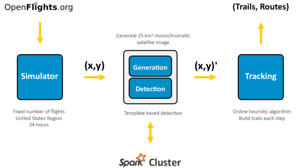
To detect all these aircraft from a world-wide image, we’ll use correlation based template matching. There are many ways to parallelize and distribute this operation, but an intuitive distributed processing of image patches will be done with each cluster node performing a parallelized Fast Fourier Transform to identify any aircraft in a given patch. Tracking will be done using an online heuristic algorithm to “connect the dots” recovered from detection. At the end of the simulation, these trails of dots will be paired with simulated routes to evaluate how well the system did.

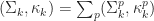
The remainder of this post will cover the architecture of the system based on Apache Spark, its configurations for running locally and on Amazon Web Services, and how well it performs before concluding with possible future work and cost analysis of what it would take to turn this into a real-world system.

System Architecture

Overview

Figure 1: Data pipeline architecture.

The system relies on the data pipeline architecture presented above. Data is read in from the OpenFlights.org dataset consisting of airport information and flight routes. A fixed number of national flights are selected and passed along to a simulation module. At each time step, the simulator identifies which airplanes to launch, update latitude and longitude coordinates, and remove those that have arrived at their destination.

To minimize the amount of network traffic being exchanged between nodes, flights are placed into buckets based on their current latitude and longitude. Buckets having flights are then processed in parallel by the Spark Workers. Each worker receives a bucket and generates a synthetic satellite image; this image is then given to the detection module which in turn recovers the coordinates from the image.

These coordinates are coalesced at the Spark Driver and passed along to the tracking module where the coordinates are appended to previously grown flight trails. Once 24 hours worth of simulated time has elapsed (in simulated 15 minute increments), the resulting tracking information is passed along to a reporting module which matches the simulated routes with the flight trails. These results are then visually inspected for quality.

Simulation Assumptions

All latitude and longitude calculations are done under the Equirectangular projection. A corresponding flight exists for each route in the OpenFlights.org dataset (Open Database License). Flights departing hourly follow a straight line trajectory between destinations. Once en route, flights are assumed to be Boeing 747s traveling at altitude of 35,000 ft with a cruising speed of 575 mph.

Generation

Figure 2: Conceptual layering and data representations between the modules of the pipeline. World silhouette by Wikimedia Commons.

Flights are mapped to one of $4000 \times 8000$ buckets based on each flight’s latitude and longitude coordinate. Each bucket spans a $0.045 \times 0.045$ degree region as illustrated in the middle layer of Fig. (2). Given a bucket, a $512 \times 512$ oversimplified synthetic medium-resolution monochromatic satellite image is created with adorning aircraft silhouettes for each $71 \times 65$ m Boeing 747 airliner in the bucket. (Visual obstructions such as clouds or nightfall will not be depicted.) This image, in addition to the latitude and longitude of the top-left and bottom-right of the image, are then passed along to the detection module.

Detection

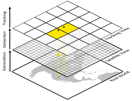
Given an image and its world coordinate frame, the detection module performs textbook Fourier-based correlation template matching to identify silhouettes of airplanes, $X$ , in the image, $Y$ :

$\displaystyle Z = \mathcal{F}^{-} \left( \mathcal{F}(X) \circ \mathcal{F}(Y) \right )$

(1)

Where the two-dimensional Discrete Fourier Transform and inverse transform are defined as:

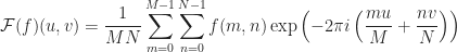$\displaystyle \mathcal{F}(f)(u,v) = \frac{1}{M N} \sum_{m = 0}^{M - 1} \sum_{n = 0}^{N - 1} f(m, n) \exp{ \left( -2 \pi i \left( \frac{mu}{M} + \frac{nv}{N} \right ) \right ) }$

(2)

$\displaystyle \mathcal{F^{-}}(F)(m,n) = \sum_{u = 0}^{M - 1} \sum_{v = 0}^{N - 1} F(u, v) \exp{ \left( 2 \pi i \left( \frac{mu}{M} + \frac{nv}{N} \right ) \right ) }$

(3)

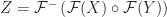
To carry out these calculations efficiently, a parallelized two-dimensional Fast Fourier Transform (FFT) $\mathcal{O}(N \log N)$ time algorithm was implemented for both forward and inverse operations by leveraging the fact that operations (2), (3) can be factored so that the FFT can be computed row-wise, and then on those results column-wise. Hadamard (element-wise) product of the frequency domain representation of the airplane and satellite image is done naively in quadratic time.

To denoise the results, the recovered spatial product, $Z$ , is thresholded so that any real values greater than 90% of the product’s real maximum, $Z^*$ , are kept:

$\displaystyle Z_{x,y} = \Re{ \left( Z_{x, y} \right ) } 1_{ [ \Re{ \left( Z_{x, y} \right ) } \ge 0.9 Z^{*} ] }$

(4)

Since there are many values greater than the threshold, a linear time (in number of nodes) connected component labeling algorithm is applied to identify the most likely aircraft locations. The algorithm treats each pixel of the image as a node if that pixel’s value is greater than the threshold. An edge exists between two nodes if the nodes’ pixel coordinates are within an $\ell_\infty$ distance of two. The centroid of each connected component is then taken to be the true coordinate of each detected aircraft. Next only those centroids derived from clusters having more than half the average number of pixels per cluster are kept. Finally, these centroids are transformed to latitude and longitude coordinates given the world coordinate frame.

Tracking

The tracking module uses an $181 \times 361$ grid of buckets with each bucket representing approximately a square degree region as illustrated as the top layer in Fig. (2). Each individual bucket consists of a stack of sightings where a sighting is a timestamped collection of coordinates. Here an individual coordinate is allowed to “connect” up to two other coordinates. Coordinates connected in this fashion form a trail, which is the primary output of the module.

Figure 3: (Left) Collinear and (Right) directional tracking heuristics. Blue points $C$ represent coordinates that would be accepted under these heuristics and red points $C^\prime$ that would be rejected.

For each latitude and longitude coordinate from the detection module, $d \in D$ , the tracking module picks all the previous time step’s coordinates, $p \in P$ , from the neighboring ( $\ell_\infty \le 5$ ) buckets of $d$ ‘s bucket. From $P$ , only those coordinates that satisfy the following criteria are considered:

$p$ must be free to “connect” to another coordinate.
$d$ must be collinear to the coordinates of the trail headed by $p$ , i.e., $\lvert AC - AB - BC \rvert \le \epsilon$ as in Fig. (3).
Given the predecessor of $p$ , the inner product of the vectors formed from the predecessor to $p$ and $d$ must be positive, i.e., $\langle \overrightarrow{AB}, \overrightarrow{AC} \rangle > 0$ as in Fig. (3).

Next, the nearest neighbor of $p$ is chosen from this remaining set of points. If a nearest neighbor exists, then $p$ is appended to the end of the nearest neighbor’s trail, otherwise a new trail is created. Finally, $p$ is added to its designated bucket so that it can be used for future trail building.

When the simulation completes, all trails from tracking module are analyzed and matched to the known routes used in the simulation. Matching is done by minimizing the distance from the trail’s origin and destination to a route’s origin and destination respectively. If the mean orthogonal distance:

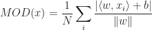$\displaystyle MOD(x) = \frac{1}{N} \sum_{i} \frac{ \lvert \langle w, x_i \rangle + b \rvert }{ \lVert w \rVert }$

(5)

from the coordinates in the trail to the line formed by connecting the route’s origin and destination is greater than 25 m, then the match is rejected.

Reporting

The reporting module is responsible for summarizing the system’s performance. The average mean orthogonal distance given by Eqn. (5) is reported for all identified routes, total number of images processed and coordinates detected, and the portion of routes correctly matched is reported.

System Configurations

Standalone

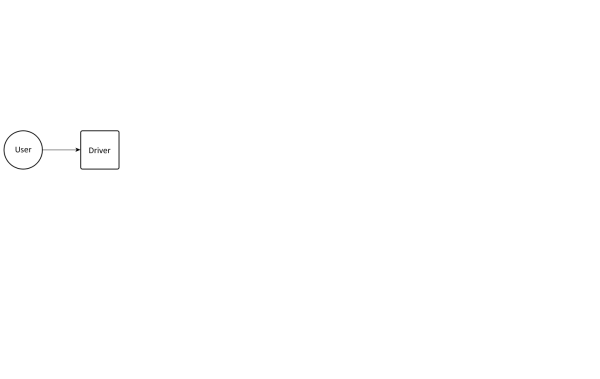
Figure 4: Standalone configuration components.

Standalone mode runs the application in a single JVM without using Spark. Experiments were ran on the quad-core Intel i7 3630QM laptop jaws, which has 8 GB of memory, 500 GB hard drive, and is running Windows 8.1 with Java SE 7.

Cluster

Figure 5: Cluster configuration components.

Cluster mode runs the application on a Spark cluster in standalone mode. Experiments were ran on a network consisting of two laptop computers connected to a private 802.11n wireless network. In addition to jaws, the laptop oddjob was used. oddjob is a quad-core Intel i7 2630QM laptop with 6 GB of memory, 500 GB hard drive running Windows 7. Atop each machine, Oracle VM VirtualBox hosts two cloned Ubuntu 14.04 guest operating systems. Each virtual machine has two cores, 2 GB of memory and a 8 GB hard drive. Each virtual machine connects to the network using a bridged network adapter to its host’s. Host and guest operating systems are running Java SE 7, Apache Hadoop 2.6, and Scala 2.11.6 as prerequisites for Apache Spark 1.3.1. In total, there are four Spark Workers who report to a single Spark Master which is driven by a single Spark Driver.

Cloud

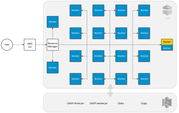
Figure 6: Cloud configuration components.

Cloud mode runs the application on an Amazon Web Services (AWS) provisioned Spark cluster managed by Apache Yarn. Experiments were ran using AWS’s Elastic Map Reduce (EMR) platform to provision the maximum allowable twenty^[1] Elastic Compute Cloud (EC2) previous generation m1.medium instances (one master, nineteen core) by scheduling jobs to execute the application JARs from the Simple Storage Service (S3). Each m1.medium instance consists of one 2 GHz CPU, 3.7 GB of memory, 3.9 GB hard drive running Amazon Machine Image (AMI) 3.6 equipped with Red Hat 4.8, Java SE 7, Spark 1.3.0. In total, there are nineteen Spark Workers and one Spark Master – one per virtual machine – managed by a Yarn Resource Manager driven by a single Yarn Client hosting the application.

System Evaluation

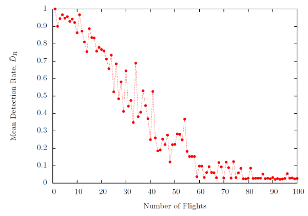
Detection Rate

Figure 7: $\overline{D}_r$ reported for flights in a single 25 km² region. Larger $\overline{D}_r$ is better.

$\displaystyle D_R = \frac{\# \left( \text{Detected coordinates} \right)}{\# \left( \text{Expected coordinates} \right)}$

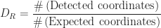(6)

When an image is sparsely populated, the system consistently detects the presence of the aircraft, however as the density increases, the system is less adapt at finding all flights in the region as shown in Fig. (7). This is unexpected behavior. Explanations include the possibility that the threshold needs to be made to be adaptive, or that a different approach needs to be taken all together. In terms of real world implications, FAA regulations (JO 7110.65V 5-4-4) state that flights must maintain a minimum lateral distance of 3 and 5 miles (4.8 to 8 km). In principle, there could be at most four flights in a given image under these guidelines and the system would still have a 96.6% chance of identifying all four positions.

Detection Accuracy

Figure 8: Detected and actual positions of a fight from Denver to Charlotte.

A flight from DIA to CTL was simulated to measure how accurate the template matching approach works as illustrated in Fig. (8). Two errors were measured: the mean orthogonal distance given by Eqn. (5) and the mean distance between the detected and actual coordinate for all time steps:

$\displaystyle MD(x, y) = \frac{1}{N} \sum_i \lVert x_i - y_i \rVert_2$

(7)

For Eqn. (5) a mean error of $9.99 \pm 3.2$ m was found, and for Eqn. (7) $19.95 \pm 3.3$ m. Both errors are acceptable given a single pixel represents approximately $10$ m. (For context, the global positioning system (GPS) has a 7.8 m error.)

Figure 9: 65% of the paired trails and routes have a MOD less than 26 m. Smaller error is better.

In terms of how accurate detection is at the macro level, 500 flights were simulated and the resulting mean orthogonal distance was analyzed. Fig. (9) illustrates the bimodal distribution that was observed. 65% of the flights observed an accuracy less than 26 m with an average accuracy of $14.2 \pm 5.8$ m, while the remaining 35% saw an average accuracy of $111.9 \pm 100$ km which is effectively being off by a full degree. It is assumed that this 35% are cases where trails are paired incorrectly with routes. Based on these findings, the system enforces that all pairings not exceed a mean orthogonal distance of 25 m.

Tracking Rate

Figure 10: $2^n$ for $n \in [0, 10]$ national fights were simulated to completion with their mean tracking rate reported over 15 trials. Larger $\overline{T}_R$ is better.

$\displaystyle T_R = \frac{\# \left( \text{Correctly paired trails} \right)}{\# \left(\text{ Expected trails} \right)}$

(8)

For Fig. (10), an increasing number of random flights were simulated to completion and the resulting mean tracking rate reported. Based on these findings, the tracking module is having difficulty correctly handling many concurrent flights originating from different airports. This behavior is likely a byproduct of how quickly the detection rate degrades when many flights occupy a single region of space. When running a similar simulation where all flights originate from the same airport, the tracking rate is consistently near-perfect independent of the number of flights. This would suggest the system has difficulty with flights that cross paths. (For context, there is on average 7,000 concurrent flights over US airspace at any given time that we would wish to track.)

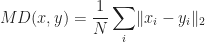
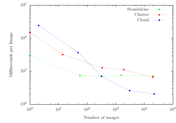
Performance

Figure 11: Average processing time per image in milliseconds for the three dierent congurations. Smaller ms/image is better.

A series of experiments was conducted against the three configurations to measure how quickly the system could process different volumes of flights across the United States over a 24-hours period. The results are illustrated in Fig. (11). Unsurprisingly, the Cloud mode outperforms both the Standalone and Cluster modes by a considerable factor as the number of flights increases.

Table 1: Processing time per image, megabytes of image data processed per second, and overall processing time for 22k images by system configuration.
Configuration	ms/image	mb/sec	Time (min)
Standalone	704	3.00	260
Cluster	670	2.84	222
Cloud	207	9.67	76

Table (1) lists the overall processing time for 22k images representing roughly 550k km², and 43 GB of image data. If the Cloud configuration was used to monitor the entire United States, then it would need approximately 22 hours to process a single snapshot consisting of 770 GB of image data. Obviously, the processing time is inadequate to keep up with a recurring avalanche of data every fifteen minutes. To do so, a real-world system would need to be capable of processing an image every 2 ms. To achieve this 1) more instances could be added, 2) the implementation can be refined to be more efficient, 3) the implementation can leverage GPUs for detection, and 4) a custom tailored alternative to Spark could be used.

Discussion

Future Work

There are many opportunities to exchange the underlying modules with more robust techniques that both scale and are able to handle real-world satellite images. The intake and generation modules can be adapted to either generate more realistic flight paths and resulting satellite imagery, or adapted to handle real-world satellite imagery from a vendor such as Skybox Imaging, Planet Labs, or DigitalGlobe.

For detection, the correlation based approach can be replaced with a cross-correlation approach, or with the more involved Scale Invariant Feature Transformation (SIFT) method which would be more robust at handling aircraft of different sizes and orientations. Alternatively, the parallelism granularity can be changed so that the two-dimensional FFT row-wise and column-wise operations are distributed over the cluster permitting the processing of larger images.

Tracking remains an open issue for this system. Getting the detection rate to be near perfect will go a long way, but the age of historical sightings considered could be increased to account for “gaps” in the detection trail. Yilmaz et al. provide an exhaustive survey of deterministic and statistical point tracking methods that can be applied here, in particular the Joint Probability Data Association Filter (JPDAF) and Multiple Hypothesis Tracking (MHT) methods which are worth exploring further.

On the reporting end of the system, a dashboard showing all of the detected trails and coordinates would provide an accessible user interface to end-users to view and analyze flight trails, discover last known locations, and detect anomalies.

Real-world Feasibility

While the scope of this work has focused on system internals, it is important to recognize that a real-world system requires a supporting infrastructure of satellites, ground stations, computing resources, facilities and staff- each of which imposes its own set of limitations on the system. To evaluate the system’s feasibility, its expected cost is compared to the expected cost of the ADS-B approach.

Following the CubeSat model and a 1970 study by J. G. Walker, 25 satellites ($1M ea.) forming a constellation in low earth orbit is needed to provide continuous whole earth coverage for $25M. Ground stations ($120k ea.) can communicate with a satellite at a time bringing total costs to $50M.^[2] Assuming that a single computer is responsible for square degree region, the system will require 64,800 virtual machines, equivalently 1,440 quad-core servers ($1k ea.) bringing the running total to $51M.

ADS-B costs are handled by aircraft owners. Average upgrade costs are $5k with prices varying by vendor and aircraft. Airports already have Universal Access Transceivers (UATs) to receive the ADS-B signals. FAA statistics list approximately 200,000 registered aircraft suggesting total cost of $1B.

Given that these are very rough estimates, an unobtrusive $51M system would be a good alternative to a $1B dollar exchange between private owners to ADS-B vendors. (Operational costs of the system were estimated to be $1.7M/year based on market rates for co-locations and staff salaries.)

Conclusions

In this work, a distributed system has been presented to detect and track commercial aircraft from synthetic satellite imagery. The system’s accuracy and detection rates are acceptable given established technologies. Given suitable hardware resources, it would be an effective tool in assisting search-and-rescue teams locate airplanes from historic satellite images. More work needs to be done to improve the system’s tracking abilities for it to be a viable real-world air traffic control system. While not implemented, the data needed to support flight deviation, flight collision detection and other air traffic control functionality is readily available. Spark is an effective tool for quickly distributing work to a cluster, but more specialized high performance computing approaches may yield better runtime performance.

References

[1] Automatic dependent surveillance-broadcast (ads-b) out equipment and use. Technical Report 14 CFR 91.225, U.S. Department of Transportation Federal Aviation Administration, May 2010.

[2] General aviation and air taxi activity survey. Technical Report Table 1.2, U.S. Department of Transportation Federal Aviation Administration, Sep 2014.

[3] Nanosats are go! The Economist, June 7 2014.

[4] A. Eisenberg. Microsatellites: What big eyes they have. New York Times, August 10 2013.

[5] A. Fasih. Machine vision. Lecture given at Transportation Informatics Group, ALPEN-ADRIA University of Klagenfurt, 2009.

[6] S. Kang, K. Kim, and K. Lee. Tablet application for satellite image processing on cloud computing platform In Geoscience and Remote Sensing Symposium (IGARSS), 2013 IEEE International, pages 1710-1712, July 2013.

[7] W. Lee, Y. Choi, K. Shon, and J. Kim. Fast distributed and parallel pre-processing on massive satellite data using grid computing. Journal of Central South University, 21(10):3850-3855, 2014.

[8] J. Lewis. Fast normalized cross-correlation. In Vision interface, volume 10, pages 120-123, 1995.

[9] W. Li, S. Xiang, H. Wang, and C. Pan. Robust airplane detection in satellite images. In Image Processing (ICIP), 2011 18th IEEE International conference on, pages 2821-2824, Sept 2011.

[10] D. G. Lowe. Distinctive image features from scale-invariant keypoints. International journal of computer vision, 60(2):91-110, 2004.

[11] H. Prajapati and S. Vij. Analytical study of parallel and distributed image processing. In Image Information Processing (ICIIP), 2011 International Conference on, pages 1-6, Nov 2011.

[12] E. L. Ray. Air traffic organization policy. Technical Report Order JO 7110.65V, U.S. Department of Transportation Federal Aviation Administration, April 2014.

[13] J. Tunaley. Algorithms for ship detection and tracking using satellite imagery. In Geoscience and Remote Sensing Symposium, 2004. IGARSS ’04. Proceedings. 2004 IEEE International, volume 3, pages 1804-1807, Sept 2004.

[14] J. G. Walker. Circular orbit patterns providing continuous whole earth coverage. Technical report, DTIC Document, 1970.

[15] Y. Yan and L. Huang. Large-scale image processing research cloud. In CLOUD COMPUTING 2014, The Fifth International Conference on Cloud Computing, GRIDs, and Virtualization, pages 88-93, 2014.

[16] A. Yilmaz, O. Javed, and M. Shah. Object tracking: A survey. Acm computing surveys (CSUR), 38(4):13, 2006.

Written by lewellen

2015-05-20 at 8:00 am

Posted in Projects

Tagged with Airplane Detection, Amazon Web Services, Apache Spark, AWS, Cloud Computing, Distributed Image Processing, Elastic Map Reduce, EMR, Grad School, Java, Object Tracking, Remote Sensing, Satellite Imagery, Template Matching

Antimatroid, The

Posts Tagged ‘AWS’

Distributed k-Means Clustering

Introduction

Background

RDMA

Barriers

Design

Dataset Transfer

Iteration and aggregation

Synchronization

Experiments

Transfer Rates

Recovery time

Runtime performance

Discussion

Related Work

Future Work

RDMA

Kernel

Barrier

Overall System

Conclusion

References

Pages

Follow by Email

Follow by RSS

Categories

Archives

Meta