C-Sharp | Antimatroid, The

Posts Tagged ‘C-Sharp’

Using GPUs to solve Spatial FitzHugh-Nagumo Equation Numerically

Introduction

Modeling Action Potentials

In neurophysiology, we wish to model how electrical impulses travel along the complex structures of neurons. In particular, along the axon since it is the principle outbound channel of the neuron. Along the axon are voltage gated ion channels in which concentrations of potassium and sodium are exchanged. During depolarization, a fast influx of sodium causes the voltage to gradually increase. During repolarization, a slow outflux of potassium causes the voltage to decrease gradually. Because the potassium gates are slow to close, there is a negative voltage dip and recovery phase afterwards called hyperpolarization.

Attempts to provide a continuous time model of these phases began with work in the 1950s by Hodgkin and Huxley [HH52]. The duo formulated a four-dimensional nonlinear system of ordinary differential equations based on an electrical circuit model of giant squid axons. This landmark contribution was later simplified in the 1960s by FitzHugh [Fit61]. Here FitzHugh casted the problem in terms of Van der Pol oscillators. This reformulation allowed him to explain the qualitative behavior of the system in terms of a two-dimensional excitation/relaxation state-space model. The following year Nagumo [NAY62] extended these equations spatially to model the desired action potential propagation along an axon, and demonstrated its behavior on analog computers. This spatial model will be the focus of this work, and a more comprehensive account of these developments can be found in [Kee02].

FitzHugh-Nagumo Equation

The Spatial FitzHugh-Nagumo equation is a two-dimensional nonlinear reaction-diffusion system:

$\displaystyle \frac{\partial }{\partial t} v = \frac{\partial^2 }{\partial^2 x} v + v \cdot (1 - v) \cdot (v - a) - w \qquad \frac{\partial }{\partial t} w = \epsilon \left( v - \gamma w \right )$
$\displaystyle v(x, 0) = v_0 \qquad w(x, 0) = 0 \qquad \frac{\partial}{\partial x} v(0, t) = 0 \qquad \frac{\partial}{\partial x} v(L, t) = 0$

(1)

Here $v(x, t)$ represents the action potential (voltage) along the axon, and $w(x, t)$ the recovery of the system. Constant $0 < a 0$ is absent from the literature, and $\epsilon > 0$ is inversely proportional to recovery time.

Mathematical Analysis

The system does not admit a general analytic solution. Mathematical analysis of the system is concerned with the existence and stability of traveling waves with [AK15] providing a thorough account of these aspects. Other analyses are concerned with the state-space model and the relationship of parameters with observed physiological behavior. In particular: self-excitatory, impulse trains, single traveling wavefronts and impulses, doubly traveling divergent wave impulses, and non-excitatory behavior that returns the system to a resting state. Since the FitzHugh-Nagumo equations are well understood, more recent literature is focused on higher dimensional and stochastic variants of the system which [Tuc13] discusses in detail.

Numerical Analysis

A survey of the literature revealed several numerical approaches to solving the FitzHugh-Nagumo equations consisting of a Finite Element method with Backward Differentiation Formulae [Ott10], and the Method of Lines [Kee02] approach. In this work, three approaches based on the Finite Difference method are investigated: an explicit scheme, an adaptive explicit scheme, and an implicit scheme; along with their associated sequential CPU bound and parallel GPU bound algorithms.

Explicit Finite Difference Scheme

To study the basic properties of the FitzHugh-Nagumo equations an explicit scheme was devised using forward and central differences for the temporal and spatial derivatives respectively.

$\displaystyle v^{j + 1}_{i} = \frac{ \Delta t }{ \Delta x^2 } \left ( v^{j}_{i+1} - 2 v^{j}_{i} + v^{j}_{i-1} \right ) + v^{j}_{i} + \Delta t \left ( v^{j}_{i} \cdot \left( 1 - v^{j}_{i} \right) \cdot \left( v^{j}_{i} - a \right ) - w^{j}_{i} \right )$
$\displaystyle w^{j+1}_{i} = \Delta t \epsilon \left( v^{j}_{i} - \gamma w^{j}_{i} \right) + w^{j}_{i}$
$\displaystyle v^{0}_{i} = v_0( i \Delta x, 0) \qquad w^{0}_{i} = 0 \qquad v^{j}_{0} = v^{j}_{1} \qquad v^{j}_{N-2} = v^{j}_{N-1}$

(2)

Truncation errors are linear in time, $\mathcal{O}(\Delta t)$ , and quadratic, $\mathcal{O}(\Delta x^{2})$ , in space. For stability, $2 \Delta t \le \Delta x^2$ , implying the use of inconveniently small time steps, however in practice it seems rare to find any mention of $\Delta x < 0.5$ in the literature. Each time step can be computed sequentially or in parallel in linear time, $\mathcal{O}(n)$ . However, there is a significant constant factor improvement delivered by parallel GPU implementations since modern GPUs allow millions of nodes to be updated in parallel giving near constant runtime performance. Further parallelization is possible by trivially distributing contiguous node sets to a combination of multiple machines and multiple GPUs.

Experiments

Figure 1: Depiction of excitation and relaxation with a constant input on the tail end of the axon. Waves travel right-to-left. State of system shown for $t = 306.19$ .

Figure 2: Impulse at $t = 0$ grows axially before its peak collapses at $t = 37.85$ giving rise to two stable impulses that travel in opposite directions before vanishing at $t = 242.98$ .

The explicit scheme was used to investigate the traveling wave and divergent wave behaviors of the FitzHugh-Nagumo equations. Fig. (1) demonstrate the application of a constant impulse, $v(t, L) = 1$ , at the end of an unexcited axon, $v_0(x) = 0$ , giving rise to oscillatory behavior. Fig. (2) shows a Gaussian impulse applied initially to the center of the axon, $v_0(x) = \exp{- \frac{(x - 100)^2}{10}}$ . As the system evolves, the impulse collapses giving rise to two separate impulses that travel in opposite directions before dissipating at the boundaries returning the axon to a completely unexcited state. Both test cases are qualitatively consistent with the literature and share the following parameters:

$\displaystyle a = 0.01 \qquad \gamma = 2 \qquad \epsilon = 0.01 \qquad N = 401 \qquad \Delta x = 0.5 \qquad 2 \Delta t < \Delta x^2$

(3)

Error Analysis

Figure 3: Varying values of $\Delta x$ w.r.t $\Delta x = 0.000045$ at $t = 0.91$ . $\Delta t$ fixed to 0.0098.

Figure 4: Varying values of $\Delta t$ w.r.t $\Delta t = 0.00023$ at different values of $t$ . $\Delta x$ fixed to 0.5.

Two experiments were ran to verify the suggested truncation errors. The numerical solution given by a sufficiently small step size serves as an analytic solution to $v(x, t)$ , which is then used to evaluate how larger steps sizes deviate as measured by the root mean squared error. Fig. (3) looks at varying $\Delta x$ and shows that as the step size as halved, the resulting RMSE is quartered consistent with the expect quadratic truncation term of the scheme. Similarly, Fig. (4) looks at varying $\Delta t$ and shows that independent of $t$ , halving the step size results in an equally reduced RMSE consistent with the expected linear truncation term of the scheme.

Runtime Performance

Figure 5: Wall time for memory allocation, memory transfers, and core loop for both CPU and GPU.

Figure 6: Wall time for just core loop for both CPU and GPU.

Comparison of sequential CPU and parallel GPU bound algorithms is based on the wall time taken to perform a single iteration to calculate $v^{j+1}$ and $w^{j+1}$ . Reported figures are a function of spatial node quantity and the mean run time of 30 iterations. The main bottleneck to performance is transferring buffers between the host and device. Fig. (5) illustrates this effect. For the largest test case considered, $N = 2^{24}$ , “GPU w/o tx” delivers 19x faster runtime over “GPU w/ tx” by not transferring intermediate results back to the host. Similarly, it delivers significantly faster runtime over the CPU by a factor of 73x. To better understand this performance boost, Fig. (6) looks at just the core loop execution time. For $N = 2^{24}$ , the core loops account for only 3.7% and 14.9% of the execution time on the CPU and GPU respectively with the GPU delivering 18x better performance than the CPU. These percentages increase monotonically, and suggest that memory transfers will eventually be dominated by sufficiently large inputs on GPUs with an abundance of memory.

Adaptive Explicit Finite Difference Scheme

While investigating the traveling wavefront solution of the system, numerical oscillations were observed as the simulation zeroed in on the steady state solution. To address this issue, an adaptive explicit scheme was devised. A survey of the literature suggested a family of moving grid methods to solve the FitzHugh-Nagumo system based on a Lagrangian formulation [VBSS90] and a method of lines formulation [Zwa11]. Here a heuristic is used to concentrate grid points where the most change takes place.

The formulation of the scheme is identical to the former section with second order spatial derivatives being approximated by Lagrange interpolating polynomials since the technique supports non-uniform grids. A three point, first order truncation error scheme is used. A five point, third order truncation error scheme was considered, but abandoned in favor of the empirically adequate three point scheme.

$\displaystyle \frac{\partial^2 }{\partial x^2} f(x_1) \approx 2 \sum_{i=0}^2 y_i \prod_{\substack{j = 0 \\ j \neq i}}^2 \frac{1}{(x_i - x_j)} + \frac{f^{(4)}(\xi_x)}{6} \left [ \prod_{\substack{i = 0 \\ i \neq 1}}^{2} (x - x_i) + 2 \sum_{\substack{i=0 \\ i \neq 1}}^{2}(x-x_i) \right ]$

(4)

The first and second spatial derivatives given by the Lagrange interpolating polynomials are used to decide how much detail is needed in the domain in addition to the first temporal derivative given by finite differences. First, a coarse grid is laid down across the entire domain to minimize the expected distance between nodes since the second order derivative has first order truncation error. Next, the magnitude of the first order spatial derivative (second order truncation error) is used to lay down a finer grid when the derivative is greater than a specified threshold. This corresponds to where the waves of the solution are.

Next, the temporal derivative is used to lay down an even finer grid in those areas having an absolute change above a specified threshold. The change in time corresponds to the dynamics of the system, by adding detail in these areas, we can preserve the behavior of the system. Finally, the zeros of the second spatial derivative serve as indicators of inflection points in the solution. These correspond most closely to the location of the traveling wavefronts of the equation. Here, the most detail is provided around a fixed radius of the inflection points since the width of the wavefronts does not depend on parameterization.

Each iteration, the explicit scheme is evaluated on the grid from the previous iteration and those results are then used to perform the grid building scheme. To map the available solution values to the new grid, the points are linearly interpolated if a new grid point falls between two previous points, or mapped directly if there is a stationary grid point between the two iterations. The latter will be the more common case since all grid points are chosen from an underlying uniform grid specified by the user. Linear interpolation will only take place when extra grid points are included in an area.

Experiments

Figure 7: Top: Numerical oscillation of a centered Gaussian impulse with $\epsilon = 0$ and all other parameters the same as those given in previous section for $t = 60.11, 90.12, 120.11$ . Bottom: Eliminated numerical oscillation based on the adaptive explicit scheme.

Fig. (7) is the motivating example for this scheme and demonstrates how numerical oscillations can be avoided by avoiding calculations in regions with stationary solutions. To demonstrate that the scheme works well for other test cases, the more interesting and dynamic divergent impulse test case is shown in Fig. (8). Here we can see that as time progresses, points are allocated to regions of the grid that are most influenced by the system’s dynamics without sacrificing quality. For the time steps shown, the adaptive scheme used 2-3x fewer nodes than the explicit scheme from the previous section.

Figure 8: Example of adaptive grid on the divergent impulse example for $t \in$ { 15.06, 30.13, 45.05, 60.12, 75.05, 90.11 }. Red lines given by the explicit scheme from the previous section, green dots given by adaptive explicit scheme.

Implicit Finite Difference Scheme

An implicit Crank-Nicolson scheme is used in this section to solve the FitzHugh-Nagumo equations. To simplify the computations, $w^{j+1}$ is solved explicitly using a second order central difference scheme before solving $v^{j+1}$ leading to the following formulation:

$\displaystyle \frac{v^{j+1}_{i}}{\Delta t} - \frac{1}{2} \left [ \frac{v^{j+1}_{i+1} - 2 v^{j+1}_{i} + v^{j+1}_{i-1}}{\Delta x^2} + v^{j+1}_{i} \left( 1 - v^{j+1}_{i} \right ) \left( v^{j+1}_{i} - a \right ) \right ]$
$\displaystyle \qquad = \frac{v^{j}_{i}}{\Delta t} + \frac{1}{2} \left [ \frac{v^{j}_{i+1} - 2 v^{j}_{i} + v^{j}_{i-1}}{\Delta x^2} + v^{j}_{i} \left( 1 - v^{j}_{i} \right ) \left( v^{j}_{i} - a \right ) \right ] + \frac{1}{2} \left [ - w^{j}_{i} - w^{j+1}_{i} \right ]$
$\displaystyle w^{j+1}_{i} = 2 \Delta t \epsilon \left( v^{j}_{i} - \gamma w^{j}_{i} \right) + w^{j-1}_{i}$
$\displaystyle v^{0}_{i} = v_0( i \Delta x, 0) \qquad w^{0}_{i} = 0 \qquad v^{j}_{0} = v^{j}_{1} \qquad v^{j}_{N-1} = v^{j}_{N-2}$

(5)

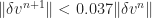
The truncation error for this scheme is $\mathcal{O}\left( \Delta t^2 + \Delta x^2 \right)$ with an improved, albeit still restrictive, requirement over the explicit scheme that $\Delta t \le \Delta x^2$ . Based on this formulation, the right-hand side is completely known when $v^{j+1}$ is calculated. This gives a simpler expression to consider:

$\displaystyle F(v^{j+1}) = LHS(v^{j+1}) - RHS = 0$

(6)

Newton’s method is used to solve the nonlinear function $F$ with an initial guess equal to the previous time step’s values, $\hat{v}^{0} = v^{n}$ . To refine the estimate, the following system is solved iteratively until the magnitude of the refinement, $\delta v$ , is less than a specified tolerance or machine epsilon.

$\displaystyle \hat{v}^{n+1} = \hat{v}^{n} - J^{-}(\hat{v}^{n}) F(\hat{v}^{n}) \qquad J(\hat{v}^{n}) \delta v = F(\hat{v}^{n}) \qquad \hat{v}^{n+1} = \hat{v}^{n} - \delta v$

(7)

This formulation gives rise to a tridiagonal Jacobian matrix, $J$ , where the first and last row are specified by no-flux boundary conditions, and constant $\alpha$ off-diagonal entries and variable $\beta_i$ diagonal entries given by the partial derivatives of each nodal equation.

$J = \begin{pmatrix} 1 & 1 & 0 & \cdots & & \\ \alpha & \beta_1 & \alpha & 0 & \cdots & \\ 0 & \alpha & \ddots & \alpha & 0 & \cdots \\ \cdots & 0 & \alpha & \ddots & \alpha & 0 \\ & \cdots & 0 & \alpha & \beta_{n-1} & \alpha \\ & & \cdots & 0 & 1 & 1 \\ \end{pmatrix}$

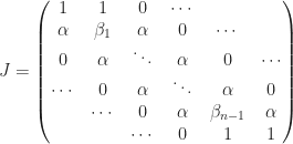
$\displaystyle \alpha = \frac{\partial}{\partial v_{i \pm 1}} F = - \frac{1}{2} \left [ \frac{1}{\Delta x^2} \right ]$

(8)

$\beta_i = \frac{\partial}{\partial v_{i}} F = \frac{1}{\Delta t} - \frac{1}{2} \left [ -\frac{2}{\Delta x^2} -3 {v_{i}}^2 + 2(1 + a) v_{i} - a \right ]$

(9)

This tridiagonal system can be solved sequentially in $\mathcal{O}(n)$ time using the Thomas algorithm or in $\mathcal{O}(n \log_2 n)$ time using the Cyclic Reduction algorithm of [Hoc65]. Cyclic Reduction begins with a forward phase in which all odd indexed unknowns are eliminated recursively until a $2 \times 2$ or $3 \times 3$ system remains that can be solved directly. Cyclic Reduction ends with a backward phase that walks up the recursion stack to solve for the previously eliminated odd indexed unknowns. Since the algorithm decouples unknowns at each recursion level of the forward and backwards phases, these reductions can be done in parallel in $\mathcal{O}(\log_2 n)$ time on the GPU assuming $n-$ fold parallelism.

Further parallelism can be achieved by solving points explicitly along the domain, then using those results to create implicit subdomains that can be solved using either Thomas or Cyclic Reduction algorithms on a combination of multiple machines and multiple GPUs at the expense of additional communication and coordination.

Error Analysis

Figure 9: Varying values of $\Delta x$ w.r.t $\Delta x = 0.012$ at $t = 0.51$ . $\Delta t$ fixed to 0.000071.

Figure 10: Varying values of $\Delta t$ w.r.t $\Delta t = 0.00025$ at different values of $t$ . $\Delta x$ fixed to 0.52.

Evaluation of the spatial error revealed an unexpected linear behavior as shown in Fig. (9). As the spatial step is halved, the resulting error was expected to become quartered, instead it is halved. No clear explanation was discovered to account for this discrepancy. With respect to time, Fig. (10) shows that both the Thomas and Cyclic Reduction algorithms were quadratic as multiple points in time were evaluated. The Thomas algorithm produced aberrations as the step size increased eventually producing numerical instability, while the Cyclic Reduction algorithm was immune to this issue.

Figure 11: Stability of implicit solvers.

Figure 12: Convergence of implicit solvers.

In terms of stability, the implicit scheme is stable up to $\Delta t \le \Delta x^2$ depending on which tridiagonal solver is used, and for comparison, the explicit scheme is stable up to precisely $2 \Delta t \le \Delta x^2$ as shown in Fig. (11). The Thomas algorithm demonstrates a slightly weaker stability guarantee than the Cyclic Reduction algorithm becoming unstable around $\Delta t / \Delta x^2 \approx 0.9$ and $\Delta t / \Delta x^2 \approx 1.05$ respectively. In terms of convergence, the Thomas algorithm typically takes more iterations than Cyclic Reduction to obtain the same degree of accuracy as shown in Fig. (12). Taking the sequence of adjustments up to machine epsilon $(2^{-52})$ , Thomas algorithm gives $\lVert \delta v^{n+1} \rVert < 0.037 \lVert \delta v^{n} \rVert$ suggesting q-linear convergence. Likewise, Cyclic Reduction gives $\lVert \delta v^{n+1} \rVert < 0.17 \lVert {\delta v^{n}}^2 \rVert$ suggesting q-quadratic convergence.

Runtime Performance

Figure 13: Performance comparison of CPU and GPU bound Thomas and Cyclic Reduction algorithms.

Figure 14: Performance comparison of Jacobian solvers.

Sequential Thomas and Cyclic Reduction routines perform equally well on CPU as shown in Fig. (13). The parallel Cyclic Reduction method did not demonstrate significant performance gains on the GPU. However, looking at just the time taken to solve the Jacobian each iteration (not including initialization or memory transfers), parallel Cyclic Reduction on the GPU was 4-5x faster than both sequential CPU solvers as shown in Fig. (14).

To explain the poor performance of Cyclic Reduction on the GPU, there are a number of different factors at play. The algorithm is susceptible to warp divergence due to the large number of conditionals that take place. Reliance on global memory access with varying strides contributes to slow performance since shared memory can’t be effectively utilized, and each iteration the adjustments are transferred from device to host to decide if Newton’s method should terminate. These different factors suggest alternative GPU implementations need to be investigated to address these different issues.

Discussion

Work Environment

All results in this paper were based on code written in C#, and compiled using Microsoft Visual Studio Express with Release settings to run on a commodity class Intel Core i7-2360QM quad core processor. Open source CUDAfy.NET is used to run C# to CUDA translated code on a commodity class NVIDIA GeForce GT 525m having two streaming multiprocessors providing 96 CUDA cores.

Future Work

Numerically, additional work could be done on the adaptive explicit scheme. In preparing the scheme, a cubic spline-based approach was abandoned in favor of simpler approaches due to time pressures. It would be worthwhile to explore how to solve the system on a spline-based “grid”.

In addition, further work could be done to optimize the implementation of the parallel Cyclic Reduction algorithm on the GPU since it delivered disappointing runtime behavior compared to the sequential algorithm on the CPU. [CmWH14] mention several different optimizations to try, and I believe better global memory access will improve runtime at the expense of more complicated addressing. As an alternative to Cyclic Reduction, both [CmWH14] and [ZCO10] detail several different parallel tridiagonal solvers that could be deployed.

In terms of models considered, there are a number of different directions that could be pursued including higher dimensional [MC04], coupled [Cat14]], [Ril06], and stochastic variants [Tuc13] of the spatial FitzHugh-Nagumo equation. Coming from a probabilistic background, I would be interested in investing time in learning how to solve stochastic ordinary and partial differential equations.

Conclusion

Three finite difference schemes were evaluated. An explicit scheme shows great performance on both the CPU and GPU, but it is susceptible to numerical oscillations. To address this issue, an adaptive explicit scheme based on heuristics was devised and is able to eliminate these issues while requiring fewer nodes to produce results on-par with the explicit scheme. An implicit scheme was evaluated which demonstrated a principled, and robust solution for a variety of test cases and is the favored approach of the three evaluated.

References

[AK15] Gianni Arioli and Hans Koch. Existence and stability of traveling pulse solutions of the fitzhugh-nagumo equation. Nonlinear Analysis: Theory, Methods and Applications, 113:51-70, 2015

[Cat14] Anna Cattani. Fitzhugh-nagumo equations with generalized diffusive coupling. Mathematical Biosciences and Engineering, 11(2):203-215, April 2014

[CmWH14] Li-Wen Chang and Wen mei W. Hwu. A guide for implementing tridiagonal solvers on gpus. In Numerical Computations with GPUs, pages 29-44. Springer International Publishing, 2014.

[Fit61] Richard FitzHugh. Impulses and physiological states in theoretical models of nerve membrane. Biophysical journal, 1(6):445, 1961.

[HH52] Alan L. Hodgkin and Andrew F. Huxley. A quantitative description of membrane current and its application to conduction and excitation in nerve. The Journal of physiology, 117(4):500-544, 1952.

[Hoc65] R. W. Hockney. A fast direct solution of poisson’s equation using fourier analysis. J. ACM, 12(1):95-113, Jan 1965.

[Kee02] James P. Keener. Spatial modeling. In Computational Cell Biology,volume 20 of Interdisciplinary Applied Mathematics, pages 171-197. Springer New York, 2002.

[MC04] Maria Murillo and Xiao-Chuan Cai. A fully implicit parallel algorithm for simulating the non-linear electrical activity of the heart. Numerical linear algebra with applications, 11(2-3):261-277, 2004.

[NAY62] J. Nagumo, S. Arimoto, and S. Yoshizawa. An active pulse transmission line simulating nerve axon. Proceedings of the IRE, 50(10):2061-2070, Oct 1962.

[Ott10] Denny Otten. Mathematical models of reaction diffusion systems, their numerical solutions and the freezing method with comsol multiphysics. 2010.

[Ril06] Caroline Jane Riley. Reaction and diffusion on the sierpinkski gasket. PhD thesis, University of Manchester, 2006.

[Tuc13] Henry C. Tuckwell. Stochastic partial differential equations in neurobiology. Linear and nonlinear models for spiking neurons. In Stochastic Biomathematical Models, volume 2058 of Lecture Notes in Mathematics. Springer Berlin Heidelberg, 2013.

[VBSS89] J. G. Verwer, J. G. Blom, and J. M. Sanz-Serna. An adaptive moving grid method for one dimensional systems of partial differential equations. Journal of Computational Physics, 82(2):454-486, 1989.

[ZCO10] Yao Zhang, Jonathan Cohen, and John D. Owens. Fast tridiagonal solvers on the gpu. SIGPLAN Not., 45(5):127-136, Jan 2010.

[Zwa11] M. N. Zwarts. A test set for an adaptive moving grid pde solver with time-dependent adaptivity. Master’s thesis. Utrecht University, Utrecht, Netherlands, 2011.

Written by lewellen

2015-11-30 at 1:58 pm

Posted in Numerical Analysis, Ordinary and Partial Differential Equations

Tagged with C-Sharp, CUDAfy.NET, Cyclic Reduction, FDM, Finite Difference Method, FitzHugh-Nagumo Equation, GPGPU, Grad School, Newton's Method, Partial Differential Equations, PDE, Reaction-Diffusion System, Tridiagonal Solver

k-Means Clustering using CUDAfy.NET

leave a comment »

Introduction

I’ve been wanting to learn how to utilize general purpose graphics processing units (GPGPUs) to speed up computation intensive machine learning algorithms, so I took some time to test the waters by implementing a parallelized version of the unsupervised k-means clustering algorithm using CUDAfy.NET– a C# wrapper for doing parallel computation on CUDA-enabled GPGPUs. I’ve also implemented sequential and parallel versions of the algorithm in C++ (Windows API), C# (.NET, CUDAfy.NET), and Python (scikit-learn, numpy) to illustrate the relative merits of each technology and paradigm on three separate benchmarks: varying point quantity, point dimension, and cluster quantity. I’ll cover the results, and along the way talk about performance and development considerations of the three technologies before wrapping up with how I’d like to utilize the GPGPU on more involved machine learning algorithms in the future.

Algorithms

Sequential

The traditional algorithm attributed to [Stu82] begins as follows:

Pick $K$ points at random as the starting centroid of each cluster.
do (until convergence)
1. For each point in data set:
  1. labels[point] = Assign(point, centroids)
2. centroids = Aggregate(points, labels)
3. convergence = DetermineConvergence()
return centroids

Assign labels each point with the label of the nearest centroid, and Aggregate updates the positions of the centroids based on the new point assignments. In terms of complexity, let’s start with the Assign routine. For each of the $N$ points we’ll compute the distance to each of the $K$ centroids and pick the centroid with the shortest distance that we’ll assign to the point. This is an example of the Nearest Neighbor Search problem. Linear search gives $\mathcal{O}( K N )$ which is preferable to using something like k-d trees which requires repeated superlinear construction and querying. Assuming Euclidean distance and points from $\mathbb{R}^d$ , this gives time complexity $\mathcal{O}( d K N )$ . The Aggregate routine will take $\mathcal{O}(d K N)$ . Assuming convergence is guaranteed in $I$ iterations then the resulting complexity is $\mathcal{O}(d K N I)$ which lends to an effectively linear algorithm.

Parallel

[LiFa89] was among the first to study several different shared memory parallel algorithms for k-means clustering, and here I will be going with the following one:

Pick $K$ points at random as the starting centroid of each cluster.
Partition $N$ points into $P$ equally sized sets
Run to completion threadId from 1 to as:
1. do (until convergence)
  1. sum, count = zero( $K * d$ ), zero( $K$ )
  2. For each point in partition[threadId]:
    1. label = Assign(point, centroids)
    2. For each dim in point:
      1. sum[ $d$ * label + dim] += point[dim]
    3. count[label] = count[label] + 1
  3. if(barrier.Synchronize())
    1. centroids = sum / count
    2. convergence = DetermineConvergence()
return centroids

The parallel algorithm can be viewed as $P$ smaller instances of the sequential algorithm processing $N/P$ chunks of points in parallel. There are two main departures from the sequential approach 1) future centroid positions are accumulated and counted after each labeling and 2) each iteration of $P$ while loops are synchronized before continuing on to the next iteration using a barrier – a way of ensuring all threads wait for the last thread to arrive, then continue to wait as the last one enters the barrier, and exits allowing the other threads to exit.

In terms of time complexity, Assign remains unchanged at $\mathcal{O}(d K)$ , and incrementing the sums and counts for the point’s label takes time $\mathcal{O}(d + 1)$ . Thus for $N/P$ points, a single iteration of the loop gives $\mathcal{O}( N/P (d K + d + 1) )$ time. Given $P$ threads, the maximum time would be given by the thread that enters the barrier, and assuming at most $I$ iterations, then the overall complexity is $\mathcal{O}(d I ( N (K + 1) + K P + 1 ) / P)$ . Which suggests we should see at most a $\mathcal{O}(K P / (K + 1))$ speedup over the sequential implementation for large values of $N$ .

GPGPU

The earliest work I found on doing k-means clustering on NVIDIA hardware in the academic literature was [MaMi09]. The following is based on that work, and the work I did above on the parallel algorithm:

Pick $K$ points at random as the starting centroid of each cluster.
Partition $N$ into $B$ blocks such that each block contains no more than $T$ points
do (until convergence)
1. Initialize sums, counts to zero
2. Process blockId 1 to , at a time in parallel on the GPGPU:
  1. If threadId == 0
    1. Initialize blockSum, blockCounts to zero
  2. Synchronize Threads
  3. label = Assign(points[blockId * $T$ + threadId], centroids)
  4. For each dim in points[blockId * + threadId]:
    1. atomic blockSum[label * pointDim + dim] += points[blockId * $T$ + threadId]
  5. atomic blockCount[label] += 1
  6. Synchronize Threads
  7. If threadId == 0
    1. atomic sums += blockSum
    2. atomic counts += blockCounts
3. centroids = sums / counts
4. convergence = DetermineConvergence()

The initialization phase is similar to the parallel algorithm, although now we need to take into account the way that the GPGPU will process data. There are a handful of Streaming Multiprocessors on the GPGPU that process a single “block” at a time. Here we assign no more than $T$ points to a block such that each point runs as a single thread to be executed on each of the CUDA cores of the Streaming Multiprocessor.

When a single block is executing we’ll initialize the running sum and count as we did in the parallel case, then request that the threads running synchronize, then proceed to calculate the label of the point assigned to the thread atomically update the running sum and count. The threads must then synchronize again, and this time only the very first thread atomically copy those block level sum and counts over to the global sum and counts shared by all of the blocks.

Let’s figure out the time complexity. A single thread in a block being executed by a Streaming Multiprocessor takes time $\mathcal{O}( 2K + (3K + 1)d + 1 )$ assuming that all $T$ threads of the block execute in parallel, that there are $B$ blocks, and $S$ Streaming Multiprocessors, then the complexity becomes: $\mathcal{O}(B / S (2K + (3K + 1)d + 1) )$ . Since $B = N / T$ , and at most $I$ iterations can go by in parallel, we are left with $\mathcal{O}( I N (2K + (3K + 1)d + 1) / T S )$ . So the expected speedup over the sequential algorithm should be $\mathcal{O}( d K T S / (2K + (3K + 1)d + 1) )$ .

Expected performance

For large values of $N$ , if we allow $K$ to be significantly larger than $d$ , we should expect the parallel version to 8x faster than the sequential version and the GPGPU version to be 255x faster than the sequential version given that $P = 8, S = 2, T = 512$ for the given set of hardware that will be used to conduct tests. For $d$ to be significantly larger than $K$ , then parallel is the same, and GPGPU version should be 340x faster than the sequential version. Now, it’s very important to point out that these are upper bounds. It is most likely that observed speedups will be significantly less due to technical issues like memory allocation, synchronization, and caching issues that are not incorporated (and difficult to incorporate) into the calculations.

Implementations

I’m going to skip the sequential implementation since it’s not interesting. Instead, I’m going to cover the C++ parallel and C# GPGPU implementations in detail, then briefly mention how scikit-learn was configured for testing.

C++

The parallel Windows API implementation is straightforward. The following will begin with the basic building blocks, then get into the high level orchestration code. Let’s begin with the barrier implementation. Since I’m running on Windows 7, I’m unable to use the convenient InitializeSynchronizationBarrier, EnterSynchronizationBarrier, and DeleteSynchronizationBarrier API calls beginning with Windows 8. Instead I opted to implement a barrier using a condition variable and critical section as follows:

// ----------------------------------------------------------------------------
// Synchronization utility functions
// ----------------------------------------------------------------------------

struct Barrier {
	CONDITION_VARIABLE conditionVariable;
	CRITICAL_SECTION criticalSection;
	int atBarrier;
	int expectedAtBarrier;
};

void deleteBarrier(Barrier* barrier) {
	DeleteCriticalSection(&(barrier->criticalSection));
	// No API for delete condition variable
}

void initializeBarrier(Barrier* barrier, int numThreads) {
	barrier->atBarrier = 0;
	barrier->expectedAtBarrier = numThreads;

	InitializeConditionVariable(&(barrier->conditionVariable));
	InitializeCriticalSection(&(barrier->criticalSection));
}

bool synchronizeBarrier(Barrier* barrier, void (*func)(void*), void* data) {
	bool lastToEnter = false;

	EnterCriticalSection(&(barrier->criticalSection));

	++(barrier->atBarrier);

	if (barrier->atBarrier == barrier->expectedAtBarrier) {
		barrier->atBarrier = 0;
		lastToEnter = true;

		func(data);

		WakeAllConditionVariable(&(barrier->conditionVariable));
	}
	else {
		SleepConditionVariableCS(&(barrier->conditionVariable), &(barrier->criticalSection), INFINITE);
	}

	LeaveCriticalSection(&(barrier->criticalSection));

	return lastToEnter;
}

A Barrier struct contains the necessary details of how many threads have arrived at the barrier, how many are expected, and structs for the condition variable and critical section.

When a thread arrives at the barrier (synchronizeBarrier) it requests the critical section before attempting to increment the atBarrier variable. It checks to see if it is the last to arrive, and if so, resets the number of threads at the barrier to zero and invokes the callback to perform post barrier actions exclusively before notifying the other threads through the condition variable that they can resume. If the thread is not the last to arrive, then it goes to sleep until the condition variable is invoked. The reason why LeaveCriticalSection is included outside the the if statement is because SleepConditionVariableCS will release the critical section before putting the thread to sleep, then reacquire the critical section when it awakes. I don’t like that behavior since its an unnecessary acquisition of the critical section and slows down the implementation.

There is a single allocation routine which performs a couple different rounds of error checking when calling calloc; first to check if the routine returned null, and second to see if it set a Windows error code that I could inspect from GetLastError. If either event is true, the application will terminate.

// ----------------------------------------------------------------------------
// Allocation utility functions
// ----------------------------------------------------------------------------

void* checkedCalloc(size_t count, size_t size) {
	SetLastError(NO_ERROR);

	void* result = calloc(count, size);
	DWORD lastError = GetLastError();

	if (result == NULL) {
		fprintf(stdout, "Failed to allocate %d bytes. GetLastError() = %d.", size, lastError);
		ExitProcess(EXIT_FAILURE);
	}

	if (result != NULL && lastError != NO_ERROR) {
		fprintf(stdout, "Allocated %d bytes. GetLastError() = %d.", size, lastError);
		ExitProcess(EXIT_FAILURE);
	}

	return result;
}

Now on to the core of the implementation. A series of structs are specified for those data that are shared (e.g., points, centroids, etc) among the threads, and those that are local to each thread (e.g., point boundaries, partial results).

// ----------------------------------------------------------------------------
// Parallel Implementation
// ----------------------------------------------------------------------------

struct LocalAssignData;

struct SharedAssignData {
	Barrier barrier;
	bool continueLoop;

	int numPoints;
	int pointDim;
	int K;

	double* points;
	double* centroids;
	int* labels;

	int maxIter;
	double change;
	double pChange;

	DWORD numProcessors;
	DWORD numThreads;

	LocalAssignData* local;
};

struct LocalAssignData {
	SharedAssignData* shared;
	int begin;
	int end;

	int* labelCount;
	double* partialCentroids;
};

The assign method does exactly what was specified in the parallel algorithm section. It will iterate over the portion of points it is responsible for, compute their labels and its partial centroids (sum of points with label $k$ , division done at aggregate step.).

void assign(int* label, int begin, int end, int* labelCount, int K, double* points, int pointDim, double* centroids, double* partialCentroids) {
	int* local = (int*)checkedCalloc(end - begin, sizeof(int));

	int* localCount = (int*)checkedCalloc(K, sizeof(int));
	double* localPartial = (double*)checkedCalloc(pointDim * K, sizeof(double));

	// Process a chunk of the array.
	for (int point = begin; point < end; ++point) {
		double optDist = INFINITY;
		int optCentroid = -1;

		for (int centroid = 0; centroid < K; ++centroid) {
			double dist = 0.0;
			for (int dim = 0; dim < pointDim; ++dim) {
				double d = points[point * pointDim + dim] - centroids[centroid * pointDim + dim];
				dist += d * d;
			}

			if (dist < optDist) {
				optDist = dist;
				optCentroid = centroid;
			}
		}

		local[point - begin] = optCentroid;
		++localCount[optCentroid];

		for (int dim = 0; dim < pointDim; ++dim)
			localPartial[optCentroid * pointDim + dim] += points[point * pointDim + dim];
	}

	memcpy(&label[begin], local, sizeof(int) * (end - begin));
	free(local);

	memcpy(labelCount, localCount, sizeof(int) * K);
	free(localCount);

	memcpy(partialCentroids, localPartial, sizeof(double) * pointDim * K);
	free(localPartial);
}

One thing that I experimented with that gave me better performance was allocating and using memory within the function instead of allocating the memory outside and using within the assign routine. This in particular was motivated after I read about false sharing where two separate threads writing to the same cache line cause coherence updates to cascade in the CPU causing overall performance to degrade. For labelCount and partialCentroids they’re reallocated since I was concerned about data locality and wanted the three arrays to be relatively in the same neighborhood of memory. Speaking of which, memory coalescing is used for the points array so that point dimensions are adjacent in memory to take advantage of caching. Overall, a series of cache friendly optimizations.

The aggregate routine follows similar set of enhancements. The core of the method is to compute the new centroid locations based on the partial sums and centroid assignment counts given by args->shared->local[t].partialCentroids and args->shared->local[t].labelCount[t]. Using these partial results all the routine to complete in $\mathcal{O}(P K d)$ time which assuming all of these parameters are significantly less than $N$ , gives a constant time routine. Once the centroids have been updated, the change in their location is computed and used to determine convergence along with how many iterations have gone by. Here if more than 1,000 iterations have occurred or the relative change in position is less than some tolerance (0.1%) then the threads will terminate.

void aggregate(void * data) {
	LocalAssignData* args = (LocalAssignData*)data;

	int* assignmentCounts = (int*)checkedCalloc(args->shared->K, sizeof(int));
	double* newCentroids = (double*)checkedCalloc(args->shared->K * args->shared->pointDim, sizeof(double));

	// Compute the assignment counts from the work the threads did.
	for (int t = 0; t < args->shared->numThreads; ++t)
		for (int k = 0; k < args->shared->K; ++k)
			assignmentCounts[k] += args->shared->local[t].labelCount[k];

	// Compute the location of the new centroids based on the work that the
	// threads did.
	for (int t = 0; t < args->shared->numThreads; ++t)
		for (int k = 0; k < args->shared->K; ++k)
			for (int dim = 0; dim < args->shared->pointDim; ++dim)
				newCentroids[k * args->shared->pointDim + dim] += args->shared->local[t].partialCentroids[k * args->shared->pointDim + dim];

	for (int k = 0; k < args->shared->K; ++k)
		for (int dim = 0; dim < args->shared->pointDim; ++dim)
			newCentroids[k * args->shared->pointDim + dim] /= assignmentCounts[k];

	// See by how much did the position of the centroids changed.
	args->shared->change = 0.0;
	for (int k = 0; k < args->shared->K; ++k)
		for (int dim = 0; dim < args->shared->pointDim; ++dim) {
			double d = args->shared->centroids[k * args->shared->pointDim + dim] - newCentroids[k * args->shared->pointDim + dim];
			args->shared->change += d * d;
		}

	// Store the new centroid locations into the centroid output.
	memcpy(args->shared->centroids, newCentroids, sizeof(double) * args->shared->pointDim * args->shared->K);

	// Decide if the loop should continue or terminate. (max iterations 
	// exceeded, or relative change not exceeded.)
	args->shared->continueLoop = args->shared->change > 0.001 * args->shared->pChange && --(args->shared->maxIter) > 0;

	args->shared->pChange = args->shared->change;

	free(assignmentCounts);
	free(newCentroids);
}

Each individual thread follows the same specification as given in the parallel algorithm section, and follows the calling convention required by the Windows API.

DWORD WINAPI assignThread(LPVOID data) {
	LocalAssignData* args = (LocalAssignData*)data;

	while (args->shared->continueLoop) {
		memset(args->labelCount, 0, sizeof(int) * args->shared->K);

		// Assign points cluster labels
		assign(args->shared->labels, args->begin, args->end, args->labelCount, args->shared->K, args->shared->points, args->shared->pointDim, args->shared->centroids, args->partialCentroids);

		// Tell the last thread to enter here to aggreagate the data within a 
		// critical section
		synchronizeBarrier(&(args->shared->barrier), aggregate, args);
	};

	return 0;
}

The parallel algorithm controller itself is fairly simple and is responsible for basic preparation, bookkeeping, and cleanup. The number of processors is used to determine the number of threads to launch. The calling thread will run one instance will the remaining $P - 1$ instances will run on separate threads. The data is partitioned, then the threads are spawned using the CreateThread routine. I wish there was a Windows API that would allow me to simultaneously create $P$ threads with a specified array of arguments because CreateThread will automatically start the thread as soon as it’s created. If lots of threads are being created, then the first will wait a long time before the last one gets around to reaching the barrier. Subsequent iterations of the synchronized loops will have better performance, but it would be nice to avoid that initial delay. After kicking off the threads, the main thread will run its own block of data, and once all threads terminate, the routine will close open handles and free allocated memory.

void kMeansFitParallel(double* points, int numPoints, int pointDim, int K, double* centroids) {
	// Lookup and calculate all the threading related values.
	SYSTEM_INFO systemInfo;
	GetSystemInfo(&systemInfo);

	DWORD numProcessors = systemInfo.dwNumberOfProcessors;
	DWORD numThreads = numProcessors - 1;
	DWORD pointsPerProcessor = numPoints / numProcessors;

	// Prepare the shared arguments that will get passed to each thread.
	SharedAssignData shared;
	shared.numPoints = numPoints;
	shared.pointDim = pointDim;
	shared.K = K;
	shared.points = points;
	
	shared.continueLoop = true;
	shared.maxIter = 1000;
	shared.pChange = 0.0;
	shared.change = 0.0;
	shared.numThreads = numThreads;
	shared.numProcessors = numProcessors;

	initializeBarrier(&(shared.barrier), numProcessors);

	shared.centroids = centroids;
	for (int i = 0; i < K; ++i) {
		int point = rand() % numPoints;
		for (int dim = 0; dim < pointDim; ++dim)
			shared.centroids[i * pointDim + dim] = points[point * pointDim + dim];
	}

	shared.labels = (int*)checkedCalloc(numPoints, sizeof(int));

	// Create thread workload descriptors
	LocalAssignData* local = (LocalAssignData*)checkedCalloc(numProcessors, sizeof(LocalAssignData));
	for (int i = 0; i < numProcessors; ++i) {
		local[i].shared = &shared;
		local[i].begin = i * pointsPerProcessor;
		local[i].end = min((i + 1) * pointsPerProcessor, numPoints);
		local[i].labelCount = (int*)checkedCalloc(K, sizeof(int));
		local[i].partialCentroids = (double*)checkedCalloc(K * pointDim, sizeof(double));
	}

	shared.local = local;

	// Kick off the threads
	HANDLE* threads = (HANDLE*)checkedCalloc(numThreads, sizeof(HANDLE));
	for (int i = 0; i < numThreads; ++i)
		threads[i] = CreateThread(0, 0, assignThread, &local[i + 1], 0, NULL);

	// Do work on this thread so that it's just not sitting here idle while the 
	// other threads are doing work.
	assignThread(&local[0]);

	// Clean up
	WaitForMultipleObjects(numThreads, threads, true, INFINITE);
	for (int i = 0; i < numThreads; ++i)
		CloseHandle(threads[i]);

	free(threads);

	for (int i = 0; i < numProcessors; ++i) {
		free(local[i].labelCount);
		free(local[i].partialCentroids);
	}

	free(local);

	free(shared.labels);

	deleteBarrier(&(shared.barrier));
}

C#

The CUDAfy.NET GPGPU C# implementation required a lot of experimentation to find an efficient solution.

In the GPGPU paradigm there is a host and a device in which sequential operations take place on the host (ie. managed C# code) and parallel operations on the device (ie. CUDA code). To delineate between the two, the [Cudafy] method attribute is used on the static public method assign. The set of host operations are all within the Fit routine.

Under the CUDA model, threads are bundled together into blocks, and blocks together into a grid. Here the data is partitioned so that each block consists of half the maximum number of threads possible per block and the total number of blocks is the number of points divided by that quantity. This was done through experimentation, and motivated by Thomas Bradley’s Advanced CUDA Optimization workshop notes [pdf] that suggest at that regime the memory lines become saturated and cannot yield better throughput. Each block runs on a Streaming Multiprocessor (a collection of CUDA cores) having shared memory that the threads within the block can use. These blocks are then executed in pipeline fashion on the available Streaming Multiprocessors to give the desired performance from the GPGPU.

What is nice about the shared memory is that it is much faster than the global memory of the GPGPU. (cf. Using Shared Memory in CUDA C/C++) To make use of this fact the threads will rely on two arrays in shared memory: sum of the points and the count of those belonging to each centroid. Once the arrays have been zeroed out by the threads, all of the threads will proceed to find the nearest centroid of the single point they are assigned to and then update those shared arrays using the appropriate atomic operations. Once all of the threads complete that assignment, the very first thread will then add the arrays in shared memory to those in the global memory using the appropriate atomic operations.

using Cudafy;
using Cudafy.Host;
using Cudafy.Translator;
using Cudafy.Atomics;
using System;

namespace CUDAfyTesting {
    public class CUDAfyKMeans {
        [Cudafy]
        public static void assign(GThread thread, int[] constValues, double[] centroids, double[] points, float[] outputSums, int[] outputCounts) {
            // Unpack the const value array
            int pointDim = constValues[0];
            int K = constValues[1];
            int numPoints = constValues[2];

            // Ensure that the point is within the boundaries of the points 
            // array.
            int tId = thread.threadIdx.x;
            int point = thread.blockIdx.x * thread.blockDim.x + tId;
            if (point >= numPoints)
                return;

            // Use two shared arrays since they are much faster than global 
            // memory. The shared arrays will be scoped to the block that this 
            // thread belongs to.

            // Accumulate the each point's dimension assigned to the k'th 
            // centroid. When K = 128 => pointDim = 2; when pointDim = 128 
            // => K = 2; Thus max(len(sharedSums)) = 256.
            float[] sharedSums = thread.AllocateShared<float>("sums", 256);
            if (tId < K * pointDim)
                sharedSums[tId] = 0.0f;

            // Keep track of how many times the k'th centroid has been assigned 
            // to a point. max(K) = 128
            int[] sharedCounts = thread.AllocateShared<int>("counts", 128);
            if (tId < K)
                sharedCounts[tId] = 0;

            // Make sure all threads share the same shared state before doing 
            // any calculations.
            thread.SyncThreads();

            // Find the optCentroid for point.
            double optDist = double.PositiveInfinity;
            int optCentroid = -1;

            for (int centroid = 0; centroid < K; ++centroid) {
                double dist = 0.0;
                for (int dim = 0; dim < pointDim; ++dim) {
                    double d = centroids[centroid * pointDim + dim] - points[point * pointDim + dim];
                    dist += d * d;
                }

                if (dist < optDist) {
                    optDist = dist;
                    optCentroid = centroid;
                }
            }

            // Add the point to the optCentroid sum
            for (int dim = 0; dim < pointDim; ++dim)
                // CUDA doesn't support double precision atomicAdd so cast down 
                // to float...
                thread.atomicAdd(ref(sharedSums[optCentroid * pointDim + dim]), (float)points[point * pointDim + dim]);

            // Increment the optCentroid count
            thread.atomicAdd(ref(sharedCounts[optCentroid]), +1);


            // Wait for all of the threads to complete populating the shared 
            // memory before storing the results back to global memory where 
            // the host can access the results.
            thread.SyncThreads();

            // Have to do a lock on both of these since some other Streaming 
            // Multiprocessor could be running and attempting to update the 
            // values at the same time.

            // Copy the shared sums to the output sums
            if (tId == 0)
                for (int i = 0; i < K * pointDim; ++i)
                    thread.atomicAdd(ref(outputSums[i]), sharedSums[i]);

            // Copy the shared counts to the output counts
            if (tId == 0)
                for (int i = 0; i < K; i++)
                    thread.atomicAdd(ref(outputCounts[i]), sharedCounts[i]);
        }

Before going on to the Fit method, let’s look at what CUDAfy.NET is doing under the hood to convert the C# code to run on the CUDA-enabled GPGPU. Within the CUDAfy.Translator namespace there are a handful of classes for decompiling the application into an abstract syntax tree using ICharpCode.Decompiler and Mono.Cecil, then converting the AST over to CUDA C via visitor pattern, next compiling the resulting CUDA C using NVIDIA’s NVCC compiler, and finally the compilation result is relayed back to the caller if there’s a problem; otherwise, a CudafyModule instance is returned, and the compiled CUDA C code it represents loaded up on the GPGPU. (The classes and method calls of interest are: CudafyTranslator.DoCudafy, CudaLanguage.RunTransformsAndGenerateCode, CUDAAstBuilder.GenerateCode, CUDAOutputVisitor and CudafyModule.Compile.)

        private CudafyModule cudafyModule;
        private GPGPU gpgpu;
        private GPGPUProperties properties;

        public int PointDim { get; private set; }
        public double[] Centroids { get; private set; }

        public CUDAfyKMeans() {
            cudafyModule = CudafyTranslator.Cudafy();

            gpgpu = CudafyHost.GetDevice(CudafyModes.Target, CudafyModes.DeviceId);
            properties = gpgpu.GetDeviceProperties(true);

            gpgpu.LoadModule(cudafyModule);
        }

The Fit method follows the same paradigm that I presented earlier with the C++ code. The main difference here is the copying of managed .NET resources (arrays) over to the device. I found these operations to be relatively time intensive and I did find some suggestions from the CUDAfy.NET website on how to use pinned memory- essentially copy the managed memory to unmanaged memory, then do an asynchronous transfer from the host to the device. I tried this with the points arrays since its the largest resource, but did not see noticeable gains so I left it as is.

At the beginning of each iteration of the main loop, the device counts and sums are cleared out through the Set method, then the CUDA code is invoked using the Launch routine with the specified block and grid dimensions and device pointers. One thing that the API does is return an array when you allocate or copy memory over to the device. Personally, an IntPtr seems more appropriate. Execution of the routine is very quick, where on some of my tests it took 1 to 4 ms to process 100,000 two dimensional points. Once the routine returns, memory from the device (sum and counts) is copied back over to the host which then does a quick operation to derive the new centroid locations and copy that memory over to the device for the next iteration.

        public void Fit(double[] points, int pointDim, int K) {
            if (K <= 0)
                throw new ArgumentOutOfRangeException("K", "Must be greater than zero.");

            if (pointDim <= 0)
                throw new ArgumentOutOfRangeException("pointDim", "Must be greater than zero.");

            if (points.Length < pointDim)
                throw new ArgumentOutOfRangeException("points", "Must have atleast pointDim entries.");

            if (points.Length % pointDim != 0)
                throw new ArgumentException("points.Length must be n * pointDim > 0.");

            int numPoints = points.Length / pointDim;

            // Figure out the partitioning of the data.
            int threadsPerBlock = properties.MaxThreadsPerBlock / 2;
            int numBlocks = (numPoints / threadsPerBlock) + (numPoints % threadsPerBlock > 0 ? 1 : 0);

            dim3 blockSize = new dim3(threadsPerBlock, 1, 1);

            dim3 gridSize = new dim3(
                Math.Min(properties.MaxGridSize.x, numBlocks),
                Math.Min(properties.MaxGridSize.y, (numBlocks / properties.MaxGridSize.x) + (numBlocks % properties.MaxGridSize.x > 0 ? 1 : 0)),
                1
                );

            int[] constValues = new int[] { pointDim, K, numPoints };
            float[] assignmentSums = new float[pointDim * K];
            int[] assignmentCount = new int[K];

            // Initial centroid locations picked at random
            Random prng = new Random();
            double[] centroids = new double[K * pointDim];
            for (int centroid = 0; centroid < K; centroid++) {
                int point = prng.Next(points.Length / pointDim);
                for (int dim = 0; dim < pointDim; dim++)
                    centroids[centroid * pointDim + dim] = points[point * pointDim + dim];
            }

            // These arrays are only read from on the GPU- they are never written 
            // on the GPU.
            int[] deviceConstValues = gpgpu.CopyToDevice<int>(constValues);
            double[] deviceCentroids = gpgpu.CopyToDevice<double>(centroids);
            double[] devicePoints = gpgpu.CopyToDevice<double>(points);

            // These arrays are written written to on the GPU.
            float[] deviceSums = gpgpu.CopyToDevice<float>(assignmentSums);
            int[] deviceCount = gpgpu.CopyToDevice<int>(assignmentCount);


            // Set up main loop so that no more than maxIter iterations take 
            // place, and that a realative change less than 1% in centroid 
            // positions will terminate the loop.
            int maxIter = 1000;
            double change = 0.0, pChange = 0.0;

            do {
                pChange = change;

                // Clear out the assignments, and assignment counts on the GPU.
                gpgpu.Set(deviceSums);
                gpgpu.Set(deviceCount);

                // Lauch the GPU portion
                gpgpu.Launch(gridSize, blockSize, "assign", deviceConstValues, deviceCentroids, devicePoints, deviceSums, deviceCount);

                // Copy the results memory from the GPU over to the CPU.
                gpgpu.CopyFromDevice<float>(deviceSums, assignmentSums);
                gpgpu.CopyFromDevice<int>(deviceCount, assignmentCount);

                // Compute the new centroid locations.
                double[] newCentroids = new double[centroids.Length];
                for (int centroid = 0; centroid < K; ++centroid)
                    for (int dim = 0; dim < pointDim; ++dim)
                        newCentroids[centroid * pointDim + dim] = assignmentSums[centroid * pointDim + dim] / assignmentCount[centroid];

                // Calculate how much the centroids have changed to decide 
                // whether or not to terminate the loop.
                change = 0.0;
                for (int centroid = 0; centroid < K; ++centroid)
                    for (int dim = 0; dim < pointDim; ++dim) {
                        double d = newCentroids[centroid * pointDim + dim] - centroids[centroid * pointDim + dim];
                        change += d * d;
                    }

                // Update centroid locations on CPU & GPU
                Array.Copy(newCentroids, centroids, newCentroids.Length);
                deviceCentroids = gpgpu.CopyToDevice<double>(centroids);

            } while (change > 0.01 * pChange && --maxIter > 0);

            gpgpu.FreeAll();

            this.Centroids = centroids;
            this.PointDim = pointDim;
        }
    }
}

Python

I include the Python implementation for the sake of demonstrating how scikit-learn was invoked throughout the following experiments section.

model = KMeans(
           n_clusters = numClusters, 
           init='random', 
           n_init = 1, 
           max_iter = 1000, 
           tol = 1e-3, 
           precompute_distances = False, 
           verbose = 0, 
           copy_x = False, 
           n_jobs = numThreads
           );

model.fit(X);    // X = (numPoints, pointDim) numpy array.

Experimental Setup

All experiments where conducted on a laptop with an Intel Core i7-2630QM Processor and NVIDIA GeForce GT 525M GPGPU running Windows 7 Home Premium. C++ and C# implementations were developed and compiled by Microsoft Visual Studio Express 2013 for Desktop targeting C# .NET Framework 4.5 (Release, Mixed Platforms) and C++ (Release, Win32). Python implementation was developed and compiled using Eclipse Luna 4.4.1 targeting Python 2.7, scikit-learn 0.16.0, and numpy 1.9.1. All compilers use default arguments and no extra optimization flags.

For each test, each reported test point is the median of thirty sample run times of a given algorithm and set of arguments. Run time is computed as the (wall) time taken to execute model.fit(points, pointDim, numClusters) where time is measured by: QueryPerformanceCounter in C++, System.Diagnostics.Stopwatch in C#, and time.clock in Python. Every test is based on a dataset having two natural clusters at .25 or -.25 in each dimension.

Results

Varying point quantity

Figure X: Left-to-right: C++, C#, Python run time to cluster 10 to 10⁷ two dimensional points in to two clusters.

Both the C++ and C# sequential and parallel implementations outperform the Python scikit-learn implementations. However, the C++ sequential and parallel implementations outperforms their C# counterparts. Though the C++ sequential and parallel implementations are tied, as it seems the overhead associated with multithreading overrides any multithreaded performance gains one would expect. The C# CUDAfy.NET implementation surprisingly does not outperform the C# parallel implementation, but does outperform the C# sequential one as the number of points to cluster increases.

So what’s the deal with Python scikit-learn? Why is the parallel version so slow? Well, it turns out I misunderstood the nJobs parameter. I interpreted this to mean that process of clustering a single set of points would be done in parallel; however, it actually means that the number of simultaneous runs of the whole process will occur in parallel. I was tipped off to this when I noticed multiple python.exe fork processes being spun off which surprised me that someone would implement a parallel routine that way leading to a more thorough reading the scikit-learn documentation. There is parallelism going on with scikit-learn, just not the desired type. Taking that into account the linear one performs reasonably well for being a dynamically typed interpreted language.

Varying point dimension

Figure X: Left-to-right: C++, C#, Python run time to cluster 10⁵, 2 to 2⁷ dimensional points in to two clusters.

The C++ and C# parallel implementations exhibit consistent improved run time over their sequential counterparts. In all cases the performance is better than scikit-learn’s. Surprisingly, the C# CUDAfy.NET implementation does worse than both the C# sequential and parallel implementations. Why do we not better CUDAfy.NET performance? The performance we see is identical to the vary point quantity test. So on one hand it’s nice that increasing the point dimensions did not dramatically increase the run time, but ideally, the CUDAfy.NET performance should be better than the sequential and parallel C# variants for this test. My leading theory is that higher point dimensions result in more data that must be transferred between host and device which is a relatively slow process. Since I’m short on time, this will have to be something I investigate in more detail in the future.

Varying cluster quantity

Figure X: Left-to-right: C++, C#, Python run time to cluster 10⁵ two dimensional points in to, 2 to 2⁷ clusters.

As in the point dimension test, the C++ and C# parallel implementations outperform their sequential counterparts, while the scikit-learn implementation starts to show some competitive performance. The exciting news of course is that varying the cluster size finally reveals improved C# CUDAfy.NET run time. Now there is some curious behavior at the beginning of each plot. We get $\le 10 \text{ ms}$ performance for two clusters, then jump up into about $\le 100 \text{ ms}$ for four to eight clusters. Number of points and their dimension are held constant, but we allocate a few extra double’s for the cluster centroids. I believe this has to do with cache behavior. I’m assuming for fewer than four clusters everything that’s needed sits nicely in the fast L1 cache, and moving up to four and more clusters requires more exchanging of data between L1, L2, L3, and (slower) memory memory to the different cores of the Intel Core i7-2630QM processor I’m using. As before, I’ll need to do some more tests to verify that this is what is truly happening.

Language comparison

Figure X: Left-to-right: point quantity, point dimension, and cluster quantity run time summaries for C++, C#, and Python implementations. Columns in yellow are the fastest observed implementation and paradigm for the given test.

For the three tests considered, the C++ implementations gave the best run time performance on point quantity and point dimension tests while the C# CUDAfy.NET implementation gave the best performance on the cluster quantity test.

The C++ implementation could be made to run faster be preallocating memory in the same fashion that C# does. In C# when an application is first created a block of memory is allocated for the managed heap. As a result, allocation of reference types in C# is done by incrementing a pointer instead of doing an unmanaged allocation (malloc, etc.). (cf. Automatic Memory Management) This allocation takes place before executing the C# routines, while the same allocation takes place during the C++ routines. Hence, the C++ run times will have an overhead not present in the C# run times. Had I implemented memory allocation in C++ the same as it’s done in C#, then the C++ implementation would be undoubtedly even faster than the C# ones.

While using scikit-learn in Python is convenient for exploratory data analysis and prototyping machine learning algorithms, it leaves much to be desired in performance; frequently coming ten times slower than the other two implementations on the varying point quantity and dimension tests, but within tolerance on the vary cluster quantity tests.

Future Work

The algorithmic approach here was to parallelize work on data points, but as the dimension of each point increases, it may make sense to explore algorithms that parallelize work across dimensions instead of points.

I’d like to spend more time figuring out some of the high-performance nuances of programming the GPGPU (as well as traditional C++), which take more time and patience than a week or two I spent on this. In addition, I’d like to dig a little deeper into doing CUDA C directly rather than through the convenient CUDAfy.NET wrapper; as well as explore OpenMP and OpenCL to see how they compare from a development and performance-oriented view to CUDA.

Python and scikit-learn were used a baseline here, but it would be worth spending extra time to see how R and Julia compare, especially the latter since Julia pitches itself as a high-performance solution, and is used for exploratory data analysis and prototyping machine learning systems.

While the emphasis here was on trying out CUDAfy.NET and getting some exposure to GPGPU programming, I’d like to apply CUDAfy.NET to the expectation maximization algorithm for fitting multivariate Gaussian mixture models to a dataset. GMMs are a natural extension of k-means clustering, and it will be good to implement the more involved EM algorithm.

Conclusions

Through this exercise, we can expect to see modest speedups over sequential implementations of about 2.62x and 11.69x in the C# parallel and GPGPU implementations respectively when attempting to find large numbers of clusters on low dimensional data. Fortunately the way you use k-means clustering is to find the cluster quantity that maximizes the Bayesian information criterion or Akaike information criterion which means running the vary centroid quantity test on real data. On the other hand, most machine learning data is of a high dimension so further testing (on a real data set) would be needed to verify it’s effectiveness in a production environment. Nonetheless, we’ve seen how parallel and GPGPU based approaches can reduce the time it takes to complete the clustering task, and learned some things along the way that can be applied to future work.

Bibliography

[LiFa89] Li Xiaobo and Fang Zhixi, “Parallel clustering algorithms”, Parallel Computing, 1989, 11(3): pp.275-290.

[MaMi09] Mario Zechner, Michael Granitzer. “Accelerating K-Means on the Graphics Processor via CUDA.” First International Conference on Intensive Applications and Services, INTENSIVE’09. pp. 7-15, 2009.

[Stu82] Stuart P. Lloyd. Least Squares Quantization in PCM. IEEE Transactions on Information Theory, 28:129-137, 1982.

Written by lewellen

2015-09-01 at 8:00 am

Posted in Algorithms

Tagged with C++, C-Sharp, CUDAfy.NET, GPGPU, k-Means Clustering, numpy, Python, scikit-learn, Windows API

Abstract Algebra in C#

Motivation

In C++ it is easy to define arbitrary template methods for computations involving primitive numeric types because all types inherently have arithmetic operations defined. Thus, a programmer need only implement one method for all numeric types. The compiler will infer the use and substitute the type at compile time and emit the appropriate machine instructions. This is C++’s approach to parametric polymorphism.

With the release of C# 2.0 in the fall of 2005, the language finally got a taste of parametric polymorphism in the form of generics. Unfortunately, types in C# do not inherently have arithmetic operations defined, so methods involving computations must use ad-hoc polymorphism to achieve the same result as in C++. The consequence is a greater bloat in code and an increased maintenance liability.

To get around this design limitation, I’ve decided to leverage C#’s approach to subtype polymorphism and to draw from Abstract Algebra to implement a collection of interfaces allowing for C++ like template functionality in C#. The following is an overview of the mathematical theory used to support and guide the design of my solution. In addition, I will present example problems from mathematics and computer science that can be represented in this solution along with examples how type agnostic computations that can be performed using this solution.

Abstract Algebra

Abstract Algebra is focused on how different algebraic structures behave in the presence of different axioms, operations and sets. In the following three sections, I will go over the fundamental sub-fields and how they are represented under the solution.

In all three sections, I will represent the distinction between algebraic structures using C# interfaces. The type parameters on these interfaces represent the sets being acted upon by each algebraic structure. This convention is consistent with intuitionistic (i.e., Chruch-style) type theory embraced by C#’s Common Type System (CTS). Use of parameter constraints will be used when type parameters are intended to be of a specific type. Functions on the set and elements of the set will be represented by methods and properties respectively.

Group Theory

Group Theory is the simplest of sub-fields of Abstract Algebra dealing with the study of a single binary operation, $(\cdot)$ , acting on a set $a, b, c \in S$ . There are five axioms used to describe the structures studied under Group Theory:

Closure: $(\cdot) : S \times S \to S$
Associativity: $(a \cdot b) \cdot c = a \cdot (b \cdot c)$
Commutativity : $a \cdot b = b \cdot a$
Identity: $a \cdot e = e \cdot a$
Inverse: $a \cdot b = e$

The simplest of these structures is the Groupoid satisfying only axiom (1). Any Groupoid also satisfying axiom (2) is known as a Semi-group. Any Semi-group satisfying axiom (4) is a Monoid. Monoid’s also satisfying axiom (5) are known as Groups. Any Group satisfying axiom (3) is an Abelian Group.

public interface IGroupoid<T> {
    T Operation(T a, T b);
}

public interface ISemigroup<T> : IGroupoid<T> {

}

public interface IMonoid<T> : ISemigroup<T> {
    T Identity { get; }
}

public interface IGroup<T> : IMonoid<T> {
    T Inverse(T t);
}

public interface IAbelianGroup<T> : IGroup<T> {

}

Ring Theory

The next logical sub-field of Abstract Algebra to study is Ring Theory which is the study of two operations, $(\cdot)$ and $(+)$ , on a single set. In addition to the axioms outlined above, there is an addition axiom for describing how one operations distributes over the other.

Distributivity: $a \cdot (b + c) = (a \cdot b) + (a \cdot c), (a + b) \cdot c = (a \cdot c) + (b \cdot c)$

All of the following ring structures satisfy axiom (6). Rings are distinguished by the properties of their operands. The simplest of these structures is the Ringoid where both operands are given by Groupoids. Any Ringoid whose operands are Semi-groups is a Semi-ring. Any Semi-ring whose first operand is a Group is a Ring. Any Ring whose second operand is a Monoid is a Ring with Unity. Any Ring with Unity whose second operand is a Group is Division Ring. Any Division Ring whose operands are both Abelian Groups is a Field.

public interface IRingoid<T, A, M>
    where A : IGroupoid<T>
    where M : IGroupoid<T> {
    A Addition { get; }
    M Multiplication { get; }

    T Distribute(T a, T b);
}

public interface ISemiring<T, A, M> : IRingoid<T, A, M>
    where A : ISemigroup<T>
    where M : ISemigroup<T> {

}

public interface IRing<T, A, M> : ISemiring<T, A, M>
    where A : IGroup<T>
    where M : ISemigroup<T> {

}

public interface IRingWithUnity<T, A, M> : IRing<T, A, M>
    where A : IGroup<T>
    where M : IMonoid<T> {

}

public interface IDivisionRing<T, A, M> : IRingWithUnity<T, A, M>
    where A : IGroup<T>
    where M : IGroup<T> {

}

public interface IField<T, A, M> : IDivisionRing<T, A, M>
    where A : IAbelianGroup<T>
    where M : IAbelianGroup<T> {

}

Module Theory

The last, and more familiar, sub-field of Abstract Algebra is Module Theory which deals with structures with an operation, $(\circ) : S \times R \to R$ , over two separate sets: $a,b \in S$ and $x,y \in R$ that satisfy the following axioms.

Distributivity of $S$ : $a \circ (x + y) = (a \circ x) + (a \circ y)$
Distributivity of $R$ : $(a + b) \circ x = (a \circ x) + (b \circ x)$
Associativity of $S$ : $a \circ (b \circ x) = (a \cdot b) \circ x$

All of the following module structures satisfy axioms (7)-(9). A Module consists of a scalar Ring and an vector Abelian Group. Any Module whose Ring is a Ring with Unity is a Unitary Module. Any Unitary Module whose Ring with Unity is a Abelian Group is a Vector Space.

public interface IModule<
    TScalar, 
    TVector, 
    TScalarRing, 
    TScalarAddativeGroup, 
    TScalarMultiplicativeSemigroup,
    TVectorAddativeAbelianGroup
>
    where TScalarRing : IRing<TScalar, TScalarAddativeGroup, TScalarMultiplicativeSemigroup>
    where TScalarAddativeGroup : IGroup<TScalar>
    where TScalarMultiplicativeSemigroup : ISemigroup<TScalar>
    where TVectorAddativeAbelianGroup : IAbelianGroup<TVector> 
{

    TScalarRing Scalar { get; }
    TVectorAddativeAbelianGroup Vector { get; }

    TVector Distribute(TScalar t, TVector r);
}

public interface IUnitaryModule<
    TScalar, 
    TVector, 
    TScalarRingWithUnity, 
    TScalarAddativeGroup, 
    TScalarMultiplicativeMonoid,
    TVectorAddativeAbelianGroup
> 
    : IModule<
        TScalar, 
        TVector, 
        TScalarRingWithUnity, 
        TScalarAddativeGroup, 
        TScalarMultiplicativeMonoid,
        TVectorAddativeAbelianGroup
    >
    where TScalarRingWithUnity : IRingWithUnity<TScalar, TScalarAddativeGroup, TScalarMultiplicativeMonoid>
    where TScalarAddativeGroup : IGroup<TScalar>
    where TScalarMultiplicativeMonoid : IMonoid<TScalar>
    where TVectorAddativeAbelianGroup : IAbelianGroup<TVector>
{

}

public interface IVectorSpace<
    TScalar,
    TVector,
    TScalarField,
    TScalarAddativeAbelianGroup,
    TScalarMultiplicativeAbelianGroup,
    TVectorAddativeAbelianGroup
>
    : IUnitaryModule<
        TScalar,
        TVector,
        TScalarField,
        TScalarAddativeAbelianGroup,
        TScalarMultiplicativeAbelianGroup,
        TVectorAddativeAbelianGroup
    >
    where TScalarField : IField<TScalar, TScalarAddativeAbelianGroup, TScalarMultiplicativeAbelianGroup>
    where TScalarAddativeAbelianGroup : IAbelianGroup<TScalar>
    where TScalarMultiplicativeAbelianGroup : IAbelianGroup<TScalar>
    where TVectorAddativeAbelianGroup : IAbelianGroup<TVector> 
{

}

Representation of Value Types

The CTS allows for both value and reference types on the .NET Common Language Infrastructure (CLI). The following are examples of how each theory presented above can leverage value types found in the C# language to represent concepts drawn from mathematics.

Enum Value Types and the Dihedral Group $D_8$

One of the simplest finite groups is the Dihedral Group of order eight, $D_{8}$ , representing the different orientations of a square, $e$ , obtained by reflecting the square about the vertical axis, $b$ , and rotating the square by ninety degrees, $a$ . The generating set is given by $\lbrace a, b \rbrace$ and gives rise to the set $\lbrace e, a, a^2, a^3, b, ba, ba^2, ba^3 \rbrace$ These elements are assigned names as follows: $\text{Rot}(0) = e$ , $\text{Rot}(90) = a$ , $\text{Rot}(180) = a^2$ , $\text{Rot}(270) = a^3$ , $\text{Ref}(\text{Ver}) = b$ , $\text{Ref}(\text{Desc}) = ba$ , $\text{Ref}(\text{Hoz}) = ba^2$ and $\text{Ref}(\text{Asc}) = ba^3$ . The relationship between these elements is visualized below:

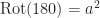
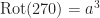
The easiest way to represent this group as a value type is with an enum.

enum Symmetry { Rot000, Rot090, Rot180, Rot270, RefVer, RefDes, RefHoz, RefAsc }

From this enum we can define the basic Group Theory algebraic structures to take us to $D_8$ .

public class SymmetryGroupoid : IGroupoid<Symmetry> {
    public Symmetry Operation(Symmetry a, Symmetry b) {
        // 64 cases
    }
}

public class SymmetrySemigroup : SymmetryGroupoid, ISemigroup<Symmetry> {

}

public class SymmetryMonoid : SymmetrySemigroup, IMonoid<Symmetry> {
    public Symmetry Identity {
        get { return Symmetry.Rot000; }
    }
}

public class SymmetryGroup : SymmetryMonoid, IGroup<Symmetry> {
    public Symmetry Inverse(Symmetry a) {
        switch (a) { 
            case Symmetry.Rot000:
                return Symmetry.Rot000;
            case Symmetry.Rot090:
                return Symmetry.Rot270;
            case Symmetry.Rot180:
                return Symmetry.Rot270;
            case Symmetry.Rot270:
                return Symmetry.Rot090;
            case Symmetry.RefVer:
                return Symmetry.RefVer;
            case Symmetry.RefDes:
                return Symmetry.RefAsc;
            case Symmetry.RefHoz:
                return Symmetry.RefHoz;
            case Symmetry.RefAsc:
                return Symmetry.RefDes;
        }

        throw new NotImplementedException();
    }

}

Integral Value Types and the Commutative Ring with Unity over $\mathbb{Z} / 2^n \mathbb{Z}$

C# exposes a number of fixed bit integral value types that allow a programmer to pick an integral value type suitable for the scenario at hand. Operations over these integral value types form a commutative ring with unity whose set is the congruence class $\mathbb{Z} / 2^n \mathbb{Z} = \lbrace \overline{0}, \overline{1}, \ldots, \overline{2^n-1} \rbrace$ where $n$ is the number of bits used to represent the integer and $\overline{m}$ is the equivalance class $\overline{m} = \lbrace m + k \cdot 2^n\rbrace$ with $k \in \mathbb{Z}$ .

Addition is given by $\overline{a} + \overline{b} = \overline{(a + b)}$ just as multiplication is given by $\overline{a} \cdot \overline{b} = \overline{(a \cdot b)}$ . Both statements are equivalent to the following congruence statements: $(a + b) \equiv c \pmod{2^n}$ and $(a \cdot b) \equiv c \pmod{2^n}$ respectively.

Under the binary numeral system, modulo $2^n$ is equivalent to ignoring the bits exceeding $n-1$ , or equivalently, $\displaystyle \sum_{i = 0}^{\infty} c_i 2^i \equiv \sum_{i = 0}^{n-1} c_i 2^i \pmod{2^n}$ where $c \in \lbrace 0, 1 \rbrace$ . As a result only the first (right most) bits need to be considered when computing the sum or product of two congruence classes, or in this case, integer values in C#. Thus, in the following implementation, it is not necessary to write any extra code to represent these operations other than writing them in their native form.

The reason why we are limited to a commutative ring with unity instead of a full field is that multiplicative inverses do not exist for all elements. A multiplicative inverse only exists when $ax \equiv 1 \pmod{2^n}$ where $x$ is the multiplicative inverse of $a$ . For a solution to exist, $\gcd(a, 2^n) = 1$ . Immediately, any even value of $a$ will not have a multiplicative inverse in $\mathbb{Z} \ 2^n \mathbb{Z}$ . However, all odd numbers will.

public class AddativeIntegerGroupoid : IGroupoid<long> {
    public long Operation(long a, long b) {
        return a + b;
    }
}

public class AddativeIntegerSemigroup : AddativeIntegerGroupoid, ISemigroup<long> {

}

public class AddativeIntegerMonoid : AddativeIntegerSemigroup, IMonoid<long> {
    public long Identity {
        get { return 0L; }
    }
}

public class AddativeIntegerGroup : AddativeIntegerMonoid, IGroup<long> {
    public long Inverse(long a) {
        return -a;
    }
}

public class AddativeIntegerAbelianGroup : AddativeIntegerGroup, IAbelianGroup<long> {

}

public class MultiplicativeIntegerGroupoid : IGroupoid<long> {
    public long Operation(long a, long b) {
        return a * b;
    }
}

public class MultiplicativeIntegerSemigroup : MultiplicativeIntegerGroupoid, ISemigroup<long> {

}

public class MultiplicativeIntegerMonoid : MultiplicativeIntegerSemigroup, IMonoid<long> {
    public long Identity {
        get { return 1L; }
    }
}

public class IntegerRingoid : IRingoid<long, AddativeIntegerGroupoid, MultiplicativeIntegerGroupoid> {
    public AddativeIntegerGroupoid Addition { get; private set;}
    public MultiplicativeIntegerGroupoid Multiplication { get; private set;}

    public IntegerRingoid() {
        Addition = new AddativeIntegerGroupoid();
        Multiplication = new MultiplicativeIntegerGroupoid();
    }

    public long Distribute(long a, long b) {
        return Multiplication.Operation(a, b);
    }
}

public class IntegerSemiring : IntegerRingoid, ISemiring<long, AddativeIntegerSemiring, MultiplicativeIntegerSemiring> {
    public AddativeIntegerSemiring Addition { get; private set;}
    public MultiplicativeIntegerSemiring Multiplication { get; private set;}

    public IntegerSemiring() : base() {
        Addition = new AddativeIntegerSemiring();
        Multiplication = new MultiplicativeIntegerSemiring();
    }
}

public class IntegerRing : IntegerSemiring, IRing<long, AddativeIntegerGroup, MultiplicativeIntegerSemigroup>{
    public new AddativeIntegerGroup Addition { get; private set; }

    public IntegerRing() : base() {
        Addition = new AddativeIntegerGroup();
    }
}

public class IntegerRingWithUnity : IntegerRing, IRingWithUnity<long, AddativeIntegerGroup, MultiplicativeIntegerMonoid> {
    public MultiplicativeIntegerMonoid Multiplication { get; private set; }

    public IntegerRingWithUnity() : base() {
        Multiplication = new MultiplicativeIntegerMonoid();
    }
}

Floating-point Value Types and the Real Vector Space $\mathbb{R}^n$

C# offers three types that approximate the set of Reals: floats, doubles and decimals. Floats are the least representative followed by doubles and decimals. These types are obviously not continuous, but the error involved in rounding calculations with respect to the calculations in question are negligible and for most intensive purposes can be treated as continuous.

As in the previous discussion on the integers, additive and multiplicative classes are defined over the algebraic structures defined in the Group and Ring Theory sections presented above. In addition to these implementations, an additional class is defined to describe a vector.

public class Vector<T> {
    private T[] vector;

    public int Dimension {
        get { return vector.Length; }
    }

    public T this[int n] {
        get { return vector[n]; }
        set { vector[n] = value; }
    }

    public Vector() {
        vector = new T[2];
    }
}

With these classes, it is now possible to implement the algebraic structures presented in the Module Theory section from above.

public class RealVectorModule : IModule<double, Vector<double>, RealRing, AddativeRealGroup, MultiplicativeRealSemigroup, VectorAbelianGroup<double>> {
    public RealRing Scalar {
        get;
        private set;
    }

    public VectorAbelianGroup<double> Vector {
        get;
        private set;
    }

    public RealVectorModule() {
        Scalar = new RealRing();
        Vector = new VectorAbelianGroup<double>(new AddativeRealAbelianGroup());
    }

    public Vector<double> Distribute(double t, Vector<double> r) {
        Vector<double> c = new Vector<double>();
        for (int i = 0; i < c.Dimension; i++)
            c[i] = Scalar.Multiplication.Operation(t, r[i]);
        return c;
    }
}

public class RealVectorUnitaryModule : RealVectorModule, IUnitaryModule<double, Vector<double>, RealRingWithUnity, AddativeRealGroup, MultiplicativeRealMonoid, VectorAbelianGroup<double>> {
    public new RealRingWithUnity Scalar {
        get;
        private set;
    }

    public RealVectorUnitaryModule()
        : base() {
        Scalar = new RealRingWithUnity();
    }
}

public class RealVectorVectorSpace : RealVectorUnitaryModule, IVectorSpace<double, Vector<double>, RealField, AddativeRealAbelianGroup, MultiplicativeRealAbelianGroup, VectorAbelianGroup<double>> {
    public new RealField Scalar {
        get;
        private set;
    }

    public RealVectorVectorSpace()
        : base() {
        Scalar = new RealField();
    }
}

Representation of Reference Types

The following are examples of how each theory presented above can leverage reference types found in the C# language to represent concepts drawn from computer science.

Strings, Computability and Monoids

Strings are the simplest of reference types in C#. From an algebraic structure point of view, the set of possible strings, $\Sigma^{*}$ , generated by an alphabet, $\Sigma$ , and paired with a concatenation operation, $(+)$ , forms a monoid.

public class StringGroupoid : IGroupoid<string> {
    public string Operation(String a, String b) {
        return string.Format("{0}{1}", a, b);
    }
}

public class StringSemigroup : StringGroupoid, ISemigroup<string> {

}

public class StringMonoid : StringSemigroup, IMonoid<string> {
    public string Identity {
        get { return string.Empty; }
    }
}

Monoids over strings have a volley of applications in the theory of computation. Syntactic Monoids describe the smallest set that recognizes a formal language. Trace Monoids describe concurrent programming by allowing different characters of an alphabet to represent different types of locks and synchronization points, while the remaining characters represent processes.

Classes, Interfaces, Type Theory and Semi-rings

Consider the set of types $\mathcal{T}^{*}$ , that are primitive and constructed in C#. The generating set of $\mathcal{T}^{*}$ is the set of primitive reference and value types, $\mathcal{T}$ , consisting of the types discussed thus far. New types can be defined by defining classes and interfaces.

A simple operation $(\oplus)$ over $\mathcal{T}^{*}$ takes two types, $\alpha, \beta$ , and yields a third type, $\gamma$ , known as a sum type. In type theory, this means that an instance of $\gamma$ can be either an instance of $\alpha$ or $\beta$ . A second operation $(\otimes)$ over $\mathcal{T}^{*}$ takes two types and yields a third type representing a tuple of the first two types. In other words, $\alpha \otimes \beta = (\alpha, \beta)$ .

Both operations form a semi-group $(\mathcal{T}^{*}, \otimes)$ and $(\mathcal{T}^{*}, \otimes)$ and in conjunction the two form a semi-ring.

To implement this semi-ring is a little involved. The .NET library supports emitting dynamic type definitions at runtime. For sum types, this would lead to an inheritance view of the operation. Types $\alpha$ and $\beta$ would end up deriving from $\gamma$ which means that any sequence of sums would yield an inheritance tree. A product type would result in composition of types with projection operations, $\pi_{n} : \prod_{i = 0} \tau_{i} \to \tau_{n}$ , to access and assign the $n\text{'th}$ element of the composite. Both type operation implementations are outside the scope of this write-up and I’ll likely revisit this topic in a future write-up.

Delegates and Process Algebras

The third type of reference type to mention is the delegate type which is C#’s approach to creating first-class functions. The simplest of delegates is the built-in Action delegate which represents a single procedure taking no inputs and returning no value.

Given actions $a, b \in \mathcal{A}$ , we can define a possible execution operator, $(\Vert) : \mathcal{A} \times \mathcal{A} \to \mathcal {A}$ , where either $a$ or $b$ is executed denoted as $a \lVert b$ . The choice operation forms a commutative semigroup $(\mathcal{A}, \lVert)$ since operations are associative $a \lVert (b \lVert c) = (a \lVert b) \lVert c$ and the operation is commutative $a \lVert b = b \lVert a$ .

A product operation, $(\to) : \mathcal{A} \times \mathcal{A} \to \mathcal {A}$ , representing the sequential execution of $a$ and then $b$ is given by $a \to b$ . The sequence operator forms a groupoid with unity since the operation is not associative $a \to (b \to c) \neq (a \to b) \to c$ and there is an identity action $e$ representing a void operation resulting in $e \to a = a$ .

Both operations together form a ringoid, $(\mathcal{A}, \to, \lVert)$ since the sequence operation distributes over the choice operation $a \to (b \lVert c) = (a \to b) \lVert (a \to c)$ . Meaning that $a$ takes place and then $b$ or $c$ takes places is equivalent to $a$ and then $b$ takes place or $a$ and then $c$ takes place.

public class SequenceGroupoidWithUnity<Action> : IGroupoid<Action> {
    public Action Identity { 
        get { return () => {}; }
    }

    public Action Operation(Action a, Action b) {
        return () => { a(); b(); }
    }
}

public class ChoiceGroupoid<Action> : IGroupoid<Action> {
    public Action Operation(Action a, Action b) {
        if(DateTime.Now.Ticks % 2 == 0)
            return a;
        return b;
    }
}

The process algebra an be extended further to describe parallel computations with an additional operation. The operations given thus far enable one to derive the possible execution paths in a process. This enables one to comprehensively test each execution path to achieve complete test coverage.

Examples

The motivation of this work was to achieve C++’s approach to parametric polymorphism by utilizing C# subtype polymorphism to define the algebraic structure required by a method (akin to the built-in operations on types in C++). To illustrate how these interfaces are to be used, the following example extension methods operate over a collection of a given type and accept the minimal algebraic structure to complete the computation. The result is a single implementation of the calculation that one would expect in C++.

static public class GroupExtensions {
    static public T Sum<T>(this IEnumerable<T> E, IMonoid<T> m) {
        return E
            .FoldL(m.Identity, m.Operation);
    }
}

static public class RingoidExtensions {
    static public T Count<T, R, A, M>(this IEnumerable<R> E, IRingWithUnity<T, A, M> r)
        where A : IGroup<T>
        where M : IMonoid<T> {

        return E
            .Map((x) => r.Multiplication.Identity)
            .Sum(r.Addition);
    }

    static public T Mean<T, A, M>(this IEnumerable<T> E, IDivisionRing<T, A, M> r)
        where A : IGroup<T>
        where M : IGroup<T> {

        return r.Multiplication.Operation(
            r.Multiplication.Inverse(
                E.Count(r)
            ),
            E.Sum(r.Addition)
        );
    }

    static public T Variance<T, A, M>(this IEnumerable<T> E, IDivisionRing<T, A, M> r)
        where A : IGroup<T>
        where M : IGroup<T> {

        T average = E.Mean(r);

        return r.Multiplication.Operation(
            r.Multiplication.Inverse(
                E.Count(r)
            ),
            E
                .Map((x) => r.Addition.Operation(x, r.Addition.Inverse(average)))
                .Map((x) => r.Multiplication.Operation(x, x) )
                .Sum(r.Addition)
        );
    }
}

static public class ModuleExtensions {
    static public TV Mean<TS, TV, TSR, TSRA, TSRM, TVA>(this IEnumerable<TV> E, IVectorField<TS, TV, TSR, TSRA, TSRM, TVA> m)
        where TSR : IField<TS, TSRA, TSRM>
        where TSRA : IAbelianGroup<TS>
        where TSRM : IAbelianGroup<TS>
        where TVA : IAbelianGroup<TV> {

        return m.Distribute(
            m.Scalar.Multiplication.Inverse(
                E.Count(m.Scalar)
            ),
            E.FoldL(
                m.Vector.Identity,
                m.Vector.Operation
            )
        );
    }
}

Conclusion

Abstract Algebra comes with a rich history and theory for dealing with different algebraic structures that are easily represented and used in the C# language to perform type agnostic computations. Several examples drawn from mathematics and computer science illustrated how the solution can be used for both value and reference types in C# and be leveraged in the context of a few example type agnostic computations. The main benefit of this approach is that it minimizes the repetitious coding of computations required under the ad-hoc polymorphism approach adopted by the designers of C# language. The downside is that several structures must be defined for the types being computed over and working with C# parameter constraint system can be unwieldy. While an interesting study, this solution would not be practical in a production setting under the current capabilities of the C# language.

References

Baeten, J.C.M. A Brief History of Process Algebra [pdf]. Department of Computer Science, Technische Universiteit Eindhoven. 31 Mar. 2012.

ECMA International. Standard ECMA-335 Common Language Infrastructure [pdf]. 2006.

Fokkink, Wan. Introduction of Process Algebra [pdf]. 2nd ed. Berlin: Springer-Verlang, 2007. 10 Apr. 2007. 31 Mar. 2012.

Goodman, Joshua. Semiring Parsing [pdf]. Computational Linguistics 25 (1999): 573-605. Microsoft Research. 31 Mar. 2012.

Hungerford, Thomas. Algebra. New York: Holt, Rinehart and Winston, 1974.

Ireland, Kenneth. A classical introduction to modern number theory. New York: Springer-Verlag, 1990.

Litvinov, G. I., V. P. Maslov, and A. YA Rodionov. Universal Algorithms, Mathematics of Semirings and Parallel Computations [pdf]. Spring Lectures Notes in Computational Science and Engineering. 7 May 2010. 31 Mar. 2012 .

Mazurkiewicz, Antoni. Introduction to Trace Theory [pdf]. Rep. 19 Nov. 1996. Institute of Computer Science, Polish Academy of Sciences. 31 Mar. 2012.

Pierce, Benjamin. Types and programming languages. Cambridge, Mass: MIT Press, 2002.

Stroustrup, Bjarne. The C++ Programming Language. Reading, Mass: Addison-Wesley, 1986.

Written by lewellen

2012-04-01 at 8:00 am

Posted in Abstract Algebra, Theoretical Computer Science

Tagged with C++, C-Sharp, Group Theory, Module Theory, Ring Theory

Space Cowboy: A Shoot’em up game in C#: Part 3

leave a comment »

Introduction

I’ve been working on a small video game the past few months and recent finished its development. You can read up on the original vision of the game and then check out how the prototype went. In this final installment of the series, I am going to present two sides of the application: the first is the layout of the application and how some of the high-level organizational aspects were implemented. The second side of the application is the gameplay and how some of the more interesting aspects were implemented. Here is a full demo of the game:

User Interface

Design

The majority of the application is based around the idea of stories and storyboards. Stories are analogous to tasks and storyboards to work flows. The transition between stories on a storyboard is initiated by the end user or by an automatic timer. The application has three main storyboards:

Main Storyboard – describes the stories that constitute the application oriented stories
Game Storyboard – defines the stories that make up the gameplay
High Scores Storyboard – how the end user interacts with the high score stories

Main Storyboard

When the user launches the game, they will be presented the Title Story. The Title Story displays the application logo and will transition to the Menu Story after a few seconds. The Menu Story displays a list of actions that the user can initiate. The user may start a new game, view the high scores, review the settings or exit the application. When the user starts a new game, they will be presented the Game Storyboard. When the user views the high scores, they will be presented the High Scores Storyboard. When the user reviews the settings, they will be presented the Settings Story. The Settings will list out all the keyboard commands. When the user exits the application, the End Title Story is displayed. The End Title Story will display the application tagline for a few seconds and then the application will terminate.

Game Storyboard

When the user elects to start a new game, the Countdown Story is displayed. The Countdown Story will display 3… 2… 1… prior to transitioning to the Gameplay Story. The Gameplay Story allows the user to play the actual game. When a user completes a level in the game, the user will be shown the Level Completed Story. The user will be able to review their performance and decide if they are done playing or want to play the next level. If they elect to quit playing, they will be taken to the High Scores Storyboard, otherwise they will be presented the Countdown Story prior to beginning the next level. If the user is destroyed and has no more lives, the user is presented the Game Over Story and after a few seconds elapses, the user will be presented the High Scores Storyboard. If a user completes all of the levels in the game, they will be presented the Game Completed Story. Similar to the Game Over Story, the Game Completed Story will transition to the High Scores Storyboard after a few seconds.

High Scores Storyboard

If a user had received a new high score during their game, they will be presented with the New High Score Story. They will enter in their name and then be transitioned to the High Scores Story. If user did not receive a new high score during their game, they will be presented the High Scores Story. The High Scores Story will display the top highest scores recorded in the game. Once the user is done reviewing the scores, they may return to the Main Storyboard. If the user had transitioned from the Main Storyboard to the High Scores Storyboard, then they will only be presented the High Scores Story.

Implementation

Each of the of storyboards is responsible for the displaying stories on the screen and transitioning between stories and storyboards (in the following I use each interchangeably). This functionality is achieved by keeping references to each story and instantiating each story on demand. When a new story is to be displayed, the storyboard will unload the current story and load up the new story. Unloading a story consists of removing the instance from the Controls collection, unregistering all event handlers and disposing of the story. Loading a story creates a new instance of the story, registers all relevant event handlers and then displays the story by adding it to the Controls collection.

To illustrate a concrete example of this practice, here is the implementation of the Main Storyboard.

using System;
using System.Windows.Forms;
using UserInterface.GameScreen.Presentation;
using UserInterface.HighScoreScreen.Presentation;
using UserInterface.HomeScreen.Presentation;
using UserInterface.Resources;
using UserInterface.SettingsScreen.Presentation;
using UserInterface.ShutdownScreen.Presentation;
using UserInterface.StartupScreen.Presentation;

namespace UserInterface {
	public class MainWindow : Form {
		private DisplayStartupStory displayStartupStory;
		private MainMenuUserControl mainMenuUserControl;
		private HighScoreStoryBoard highScoreStoryBoard;
		private DisplaySettingsStory displaySettingsStory;
		private GameStoryBoard gameStoryBoard;
		private DisplayShutdownStory displayShutdownStory;

		public MainWindow() {
			base.Width = 320;
			base.Height = 480;
			base.FormBorderStyle = FormBorderStyle.FixedSingle;
			base.MaximizeBox = false;
			base.SizeGripStyle = SizeGripStyle.Hide;
			base.BackColor = InMemoryResources.BackgroundColor;
			base.Text = "Space Cowboy";
			base.Icon = InMemoryResources.LogoIcon;
		}

		protected override void OnLoad(EventArgs e) {
			base.OnLoad(e);
			this.Location = this.DesktopLocation = new System.Drawing.Point(400, 100);
			loadStartup();
		}

		private void handleStartupDisplayed() {
			unloadStartup();
			loadMenu();
		}

		private void handleNewGame() {
			unloadMenu();
			loadGame();
		}

		private void handleGameOver(int score) {
			unloadGame();
			loadHighScores(score);
		}

		private void handleShowHighScores() {
			unloadMenu();
			loadHighScores(null);
		}

		private void handleHighscoreShowMenu() {
			unloadHighScores();
			loadMenu();
		}

		private void handleShowSettings() {
			unloadMenu();
			loadSettings();
		}

		private void handleSettingsShowMenu() {
			unloadSettings();
			loadMenu();
		}

		private void handleExit() {
			unloadMenu();
			loadShutdown();
		}

		private void handleShutdownDisplayed() {
			unloadShutdown();
			Application.Exit();
		}

		private void loadStartup() {
			displayStartupStory = new DisplayStartupStory();
			displayStartupStory.Dock = DockStyle.Fill;
			displayStartupStory.Displayed += new Action(handleStartupDisplayed);
			Controls.Add(displayStartupStory);
		}

		private void unloadStartup() {
			Controls.Clear();
			displayStartupStory.Displayed -= handleStartupDisplayed;
			displayStartupStory.Dispose();
			displayStartupStory = null;
		}

		
		private void loadMenu() {
			mainMenuUserControl = new MainMenuUserControl();
			mainMenuUserControl.Dock = DockStyle.Fill;
			mainMenuUserControl.NewGame += new Action(handleNewGame);
			mainMenuUserControl.ShowHighScores += new Action(handleShowHighScores);
			mainMenuUserControl.ShowSettings += new Action(handleShowSettings);
			mainMenuUserControl.Exit += new Action(handleExit);
			Controls.Add(mainMenuUserControl);
		}
	
		private void unloadMenu() {
			Controls.Clear();
			mainMenuUserControl.NewGame -= handleNewGame;
			mainMenuUserControl.ShowHighScores -= handleShowHighScores;
			mainMenuUserControl.ShowSettings -= handleShowSettings;
			mainMenuUserControl.Exit -= handleExit;
			mainMenuUserControl.Dispose();
			mainMenuUserControl = null;
		}


		private void loadGame() {
			gameStoryBoard = new GameStoryBoard();
			gameStoryBoard.Dock = DockStyle.Fill;
			gameStoryBoard.GameOver += new Action<int>(handleGameOver);
			Controls.Add(gameStoryBoard);
		}

		private void unloadGame() {
			Controls.Clear();
			gameStoryBoard.GameOver -= handleGameOver;
			gameStoryBoard.Dispose();
			gameStoryBoard = null;
		}


		private void loadHighScores(int? score) {
			highScoreStoryBoard = (score == null) ? new HighScoreStoryBoard() : new HighScoreStoryBoard(score.Value);
			highScoreStoryBoard.ShowMenu += new Action(handleHighscoreShowMenu);
			highScoreStoryBoard.Dock = DockStyle.Fill;
			Controls.Add(highScoreStoryBoard);
		}

		private void unloadHighScores() {
			Controls.Clear();
			highScoreStoryBoard.ShowMenu -= handleHighscoreShowMenu;
			highScoreStoryBoard.Dispose();
			highScoreStoryBoard = null;
		}


		private void loadSettings() {

			displaySettingsStory = new DisplaySettingsStory();
			displaySettingsStory.ShowMenu += new Action(handleSettingsShowMenu);
			displaySettingsStory.Dock = DockStyle.Fill;
			Controls.Add(displaySettingsStory);
		}

		private void unloadSettings() {
			Controls.Clear();
			displaySettingsStory.ShowMenu -= handleSettingsShowMenu;
			displaySettingsStory.Dispose();
			displaySettingsStory = null;
		}


		private void loadShutdown() {
			displayShutdownStory = new DisplayShutdownStory();
			displayShutdownStory.Dock = DockStyle.Fill;
			displayShutdownStory.Displayed += new Action(handleShutdownDisplayed);
			Controls.Add(displayShutdownStory);
		}

		private void unloadShutdown() {
			Controls.Clear();
			displayShutdownStory.Displayed -= handleShutdownDisplayed;
			displayShutdownStory.Dispose();
			displayShutdownStory = null;
		}
	}
}

A typical story contains a few controls and a sparse amount of logic. The following is the Game Story and a custom control called the LevelCanvas which is responsible for drawing the actors of the universe on the screen. The LevelCanvas derives from a custom control that uses a manual double buffering scheme that I’ve written about in some of my previous posts.

using System.Windows.Forms;
using UserInterface.GameScreen.Gameplay;

namespace UserInterface.GameScreen.Presentation {
	public class GameStory : UserControl {
		private TableLayoutPanel panel;
		private GameStatisticsView headsUpDisplay;
		private LevelCanvas levelUserControl;

		public GameStory(Game game) {
			headsUpDisplay = new GameStatisticsView(game.GameStatistics);
			headsUpDisplay.Dock = DockStyle.Fill;

			levelUserControl = new LevelCanvas(game);
			levelUserControl.Dock = DockStyle.Fill;

			panel = new TableLayoutPanel();
			panel.ColumnStyles.Add(new ColumnStyle() { SizeType = SizeType.Percent, Width = 100.0f });
			panel.RowStyles.Add(new RowStyle() { SizeType = SizeType.Absolute, Height = 48.0f });
			panel.RowStyles.Add(new RowStyle() { SizeType = SizeType.Percent, Height = 100.0f });
			panel.Dock = DockStyle.Fill;
			panel.Controls.Add(headsUpDisplay, 0, 0);
			panel.Controls.Add(levelUserControl, 0, 1);

			Controls.Add(panel);
		}
	}

	public class LevelCanvas : DoubleBufferedUserControl {
		private Game game;
		private Level currentLevel;

		public LevelCanvas(Game game) {
			this.game = game;

			this.BorderStyle = BorderStyle.FixedSingle;

			game.StartLevel += new Action<Level>(handleStartLevel);
			game.LevelCompleted += new Action<SessionStatistics>(handleLevelCompleted);
			game.LevelOver += new Action(handleLevelOver);
		}

		override protected void Dispose(bool disposing) {
			base.Dispose(disposing);

			if (disposing) {
				game.StartLevel -= handleStartLevel;
				game.LevelCompleted -= handleLevelCompleted;
				game.LevelOver -= handleLevelOver;
			}
		}

		override protected void Draw(Graphics graphics) {
			if (currentLevel == null)
				return;

			graphics.InterpolationMode = InterpolationMode.Bicubic;
			graphics.PixelOffsetMode = PixelOffsetMode.HighSpeed;
			graphics.SmoothingMode = SmoothingMode.AntiAlias;

			foreach (Actor actor in currentLevel.Actors) {
				try {
					actor.View.Draw(graphics, ClientRectangle);
				} catch (Exception E) {
					System.Diagnostics.Trace.WriteLine(E);
				}
			}
		}

		private void handleLevelChanged() {
			if (InvokeRequired) {
				Invoke(new Action(handleLevelChanged));
				return;
			}

			Draw();
		}

		private void handleLevelCompleted(SessionStatistics statistics) {
			if (InvokeRequired) {
				Invoke(new Action<SessionStatistics>(handleLevelCompleted), statistics);
				return;
			}

			currentLevel.Stop();
			currentLevel.LevelChanged -= handleLevelChanged;
			currentLevel = null;

			Invalidate();
		}

		private void handleLevelOver() {
			if (InvokeRequired) {
				Invoke(new Action(handleLevelOver));
				return;
			}

			currentLevel.Stop();
			currentLevel.LevelChanged -= handleLevelChanged;
			currentLevel = null;

			Invalidate();
		}

		private void handleStartLevel(Level level) {
			if (InvokeRequired) {
				Invoke(new Action<Level>(handleStartLevel));
				return;
			}

			currentLevel = level;
			currentLevel.LevelChanged += new Action(handleLevelChanged);
			currentLevel.User.Behavior = new KeyboardActorBehavior(currentLevel, this);

			currentLevel.Start();

			Invalidate();
		}
	}
}

Gameplay

Design

Much of the gameplay design was focused on providing a positive end user experience. The end user experience revolves around making the gameplay predictable, so that the end user could learn how to play quickly, then shifts to introduce new dynamics keeping the experience fresh. The core concepts that constitute the end user experience can be summarized as:

Mechanics – how things in the game universe behave
Incentives – making the end user want to play the game again and again
Extras – making the game more interesting and requiring new strategies

Mechanics

The end user is given the ability to maneuver about the universe and to fire weapons. The user is able to issue commands to move the ship north, east, south or west. Each command results in a small amount of thrust being produced
A user can rotate the ship’s weapons to the target an object in the universe and engage the weapons to emit projectiles. Projectiles follow the same rules as every other object in the universe
The user is given a fixed number of health points. Each time a ship collides with another object in the universe, both objects have their health depleted by a fixed amount. If the total points goes to zero, the user has two additional lives to use. Once all the lives have been used up, the game is over
All enemies in the universe will attempt to destroy the user at all costs

Incentives

Each time a user destroys an object in the universe, they may receive a variable amount of points that contributes to their overall score

Extras

The head-up display will flash and then fade back to normal whenever a value changes
An object’s overall health can be determined by the object’s opacity on the screen. A completely healthy object will be full opaque and the closer an object is to be destroyed, the more transparent it will appear
When an object is destroyed, it may reveal power-ups that were hidden inside or breakup into smaller pieces of debris. Power-ups come in the following flavors:
- Health – Set’s the object’s health to 100%
- Engine – Increases the propulsion of the object’s engine
- Weapon – Replaces the standard weapon with three standard weapons

Implementation

Game state

The Level class is responsible for driving the game in terms of notifying the UI to redraw the universe and for evolving the universe according to the design rules. The main method of interest is the handleTick method, which is responsible for running through the objects in the universe and then firing off different events based on the state of the universe. The class also takes care of the process of breaking an object into debris and applying non-physical behavior to collisions.

using System;
using System.Collections.Generic;
using Library.Mathematics;
using UserInterface.GameScreen.Gameplay.Behavior;
using UserInterface.GameScreen.Physics;

namespace UserInterface.GameScreen.Gameplay {
	public class Level {
		static private Random RNG;

		static Level() {
			RNG = new Random((int)(DateTime.Now.Ticks & 0xffffff));
		}

		public event Action LevelChanged;
		public event Action<SessionStatistics> LevelCompleted;
		public event Action UserDestroyed;
		public event Action<int> UserScored;

		private LevelStatistics levelStatistics;
		private TimePiece timePiece;
		private PhysicsEngine physicsEngine;
		
		public List<Actor> Actors { get; protected set; }
		public UserActor User { get; protected set; }

		public Level(double width, double height) {
			physicsEngine = new PhysicsEngine(width, height);
			physicsEngine.Collided += new Action<Actor, Actor>(handleCollided);

			levelStatistics = new LevelStatistics();

			timePiece = new TimePiece();
			timePiece.Tick += new Action(handleTick);

			User = new UserActor();
			Actors = new List<Actor>() { User };
		}

		public void Start() {
			timePiece.Start();
		}

		public void Stop() {
			timePiece.Stop();
		}

		private List<Actor> breakUp(Actor actor) {
			List<Actor> actors = new List<Actor>();
			if (actor.Body.Radius <= 6)
				return actors;

			if (actor.GetType().Equals(typeof(PowerUpNeutralActor)))
				return actors;

			for (int n = 0; n < 3; n++) {
				Actor fragment = null;

				if (0.4 * actor.Body.Radius == 6.0) {
					int x = RNG.Next(0, 10);
					if (x == 0) {
						fragment = new HealthPowerUpNeutralActor();
					} else if (x == 1) {
						fragment = new EnginePowerUpNeutralActor();
					} else if (x == 2) {
						fragment = new WeaponPowerUpNeutralActor();
					} else {
						fragment = new DebrisNeutralActor();
					}
				} else {
					fragment = new DebrisNeutralActor();
				}

				fragment.Body = new Body() {
					CurrentMass = 0.1 * actor.Body.StartingMass,
					Radius = 0.4 * actor.Body.Radius
				};

				fragment.AngularMovement = new AngularMovement() {
					Acceleration = actor.AngularMovement.Acceleration,
					Heading = actor.AngularMovement.Heading,
					Velocity = actor.AngularMovement.Velocity
				};


				fragment.LinearMovement = new LinearMovement() {
					Acceleration = new Vector(2, (i) => actor.LinearMovement.Acceleration[i]),
					Location = new Vector(2, (i) => actor.LinearMovement.Location[i]),
					Velocity = new Vector(2, (i) => actor.LinearMovement.Velocity[i])
				};

				fragment.Points = 0;

				fragment.Behavior = new MeanderActorBehavior(fragment);

				Vector direction = new Vector(2);
				direction[0] = Math.Cos((n * 120.0) * (Math.PI / 180.0));
				direction[1] = Math.Sin((n * 120.0) * (Math.PI / 180.0));

				fragment.LinearMovement.Location += (actor.Body.Radius * 0.5) * direction;
				fragment.LinearMovement.Velocity = (0.3 * actor.LinearMovement.Velocity.Length()) * direction;

				actors.Add(fragment);
			}

			return actors;
		}

		private void handleCollided(Actor A, Actor B) {
			bool aIsPowerUp = A is PowerUpNeutralActor;
			bool bIsPowerUp = B is PowerUpNeutralActor;
			if (!(aIsPowerUp ^ bIsPowerUp))
				return;

			PowerUpNeutralActor powerUpActor = null;
			Actor receipentActor = null;
			if (aIsPowerUp) {
				powerUpActor = A as PowerUpNeutralActor;
				receipentActor = B;
			} else {
				powerUpActor = B as PowerUpNeutralActor;
				receipentActor = A;
			}

			if (receipentActor is BulletUserActor || receipentActor is BulletEnemyActor)
				return;

			powerUpActor.Apply(receipentActor);
		}

		private void handleTick() {
			physicsEngine.Step(0.1, Actors);

			List<Actor> actorsToAdd = new List<Actor>();
			for (int n = 0; n < Actors.Count; n++) {

				if (Actors[n].Body.CurrentMass <= 0.0) {
					if (Actors[n].Equals(User)) {
						userDestroyed();
					} else {
						if (Actors[n] is BulletUserActor || Actors[n] is BulletEnemyActor) {

						} else {
							userScored(Actors[n].Points);
							actorsToAdd.AddRange(breakUp(Actors[n]));
						}

						Actors.RemoveAt(n--);
					}
				}
			}
			Actors.AddRange(actorsToAdd);

			if (isLevelComplete())
				levelCompleted();

			int actorCount = Actors.Count;
			for (int n = 0; n < actorCount; n++)
				Actors[n].Step(0.1);

			levelChanged();
		}

		private bool isLevelComplete() {
			for (int n = 0; n < Actors.Count; n++) {
				if (Actors[n] is BulletEnemyActor || Actors[n] is BulletUserActor)
					continue;

				if (Actors[n] is EnemyActor || Actors[n] is NeutralActor)
					return false;
			}
			return true;
		}

		private void levelChanged() {
			if (LevelChanged != null)
				LevelChanged();
		}

		private void levelCompleted() {
			if (LevelCompleted != null) {
				levelStatistics.TimeTaken = TimeSpan.FromMilliseconds(timePiece.ElapsedTimeMilliseconds);
				LevelCompleted(new SessionStatistics() {
					LevelStatistics = levelStatistics
				});
			}
		}

		private void userDestroyed() {
			levelStatistics.LivesLost++;

			if (UserDestroyed != null)
				UserDestroyed();
		}

		private void userScored(int points) {
			levelStatistics.Scored += points;

			if (UserScored != null)
				UserScored(points);
		}
	}
}

Physics

One of the key features of the game is providing a realistic enough perception of a simulated universe and that the user is able to interact with objects. This is done by providing a handful of basic physical attributes that are implemented by the PhysicsEngine class. The core responsibilities of the class is to apply physical rules over the course of a slice of time. Objects in the universe can be destroyed and created during this process.

Collisions between actors is handled through the typical conservation of linear momentum approach. Two objects, $A$ and $B$ , with momentums, $p_{A}$ and $p_{B}$ , must have the same amount of momentum before and after the collision. Assuming a totally elastic collision, we end up with $p_{A}^{(b)} + p_{B}^{(b)} = p_{A}^{(a)} + p_{B}^{(a)}$ . Momentum is defined as $p = \frac{1}{2} m v^{2}$ , where $m$ is the mass of an object and $v$ is its velocity. Since no mass is being lost in the collision, the velocities must change as a result. Solving for the $v^{(a)}$ velocities yields the trajectories that the objects will follow after the collision.

Collisions between actors and walls is once again handled through the typical conservation of momentum. Since the wall is of infinite mass and has zero velocity, the colliding object’s velocity is reflected about the wall’s normal vector.

Any object that escapes or has invalid numerical data is removed from the universe.

using System;
using System.Collections.Generic;
using Library.Mathematics;

namespace UserInterface.GameScreen.Physics {
	public class PhysicsEngine {
		public event Action<Actor, Actor> Collided;

		private double Width, Height;

		public PhysicsEngine(double width, double height) {
			Width = width;
			Height = height;
		}

		public void Step(double dt, List<Actor> actors) {
			// Actor-Actor interactions
			for (int n = 0; n < actors.Count; n++)
				for (int m = n + 1; m < actors.Count; m++)
					if (intersects(actors[n], actors[m])) {
						collide(actors[n], actors[m]);
					}

			// Actor-Wall interactions
			for (int n = 0; n < actors.Count; n++) {
				Vector l = actors[n].LinearMovement.Location;
				Vector v = actors[n].LinearMovement.Velocity;
				double r = actors[n].Body.Radius;

				if (l[0] - r < 0)
					l[0] = r;

				if (l[0] + r > Width)
					l[0] = Width - r;

				if (l[1] - r < 0)
					l[1] = r;

				if (l[1] + r > Height)
					l[1] = Height - r;

				Vector N = getWallNormal(l, r);
				if (N != null)
					actors[n].LinearMovement.Velocity = v - (2 * N.dot(v)) * N;
			}

			// get rid of anything that escaped the universe.
			for (int n = 0; n < actors.Count; n++) {
				Vector l = actors[n].LinearMovement.Location;
				double r = actors[n].Body.Radius;

				if (double.IsInfinity(l[0]) || double.IsInfinity(l[1])) {
					actors.RemoveAt(n--);
					continue;
				}

				if (double.IsNaN(l[0]) || double.IsNaN(l[1])) {
					actors.RemoveAt(n--);
					continue;
				}

				if (l[0] - r < -5 || l[0] + r > Width + 5 || l[1] - r < -5 || l[1] + r > Height + 5)
					actors.RemoveAt(n--);
			}
		}

		private bool intersects(Actor A, Actor B) {
			Vector pointDistance = (A.LinearMovement.Location - B.LinearMovement.Location);
			double touchingPointDistance = (A.Body.Radius + B.Body.Radius);
			return pointDistance.Length() <= touchingPointDistance;
		}

		private void collide(Actor A, Actor B) {
			Vector a = (1.0 / (A.Body.CurrentMass + B.Body.CurrentMass)) * ((A.Body.CurrentMass - B.Body.CurrentMass) * A.LinearMovement.Velocity + (2 * B.Body.CurrentMass) * B.LinearMovement.Velocity);
			Vector b = (1.0 / (A.Body.CurrentMass + B.Body.CurrentMass)) * ((B.Body.CurrentMass - A.Body.CurrentMass) * B.LinearMovement.Velocity + (2 * A.Body.CurrentMass) * A.LinearMovement.Velocity);

			A.LinearMovement.Velocity = a;
			B.LinearMovement.Velocity = b;

			A.Body.CurrentMass -= 2.5;
			B.Body.CurrentMass -= 2.5;

			if (Collided != null)
				Collided(A, B);
		}

		private Vector getWallNormal(Vector l, double r) {
			Vector N = null;
			if (l[0] - r <= 0.0) {
				// left side of the body is against the left side of the frame
				if (l[1] - r <= 0.0) {
					// top of the body is against the top of the frame
					// => two point of contact
					N = new Vector(2, (i) => i == 0 ? 1 : -1);
				} else if (l[1] + r >= Height) {
					// bottom of the body is against the bottom of the frame
					// => two points of contact
					N = new Vector(2, (i) => i == 0 ? 1 : 1);
				} else {
					// body is between the top and bottom
					// => single point of contact
					N = new Vector(2, (i) => i == 0 ? 1 : 0);
				}
			} else if (l[0] + r >= Width) {
				// right side of the body is against the right side of the frame
				if (l[1] - r <= 0.0) {
					// top of the body is against the top of the frame
					// => two points of contact
					N = new Vector(2, (i) => i == 0 ? -1 : -1);
				} else if (l[1] + r >= Height) {
					// bottom of the body is against the bottom of the frame
					// => two points of contact
					N = new Vector(2, (i) => i == 0 ? -1 : 1);
				} else {
					// body is between the top and bottom
					// => single point of contact
					N = new Vector(2, (i) => i == 0 ? -1 : 0);
				}
			} else {
				// body is between the left and right
				if (l[1] - r <= 0.0) {
					// top of the body is against the top of the frame
					// => single point of contact
					N = new Vector(2, (i) => i == 1 ? -1 : 0);
				} else if (l[1] + r >= Height) {
					// bottom of the body is against the bottom of the frame
					// => single point of contact
					N = new Vector(2, (i) => i == 1 ? +1 : 0);
				} else {
					// body is between the top and bottom
					// => zero points of contact
				}
			}
			return N;
		}
	}
}

Enemy Targeting

To make the game more interesting, the enemy ships are able to target the user’s ship. Since the enemy must adhere to the same mechanics that the user does, it incrementally rotates clockwise and counterclockwise to keep the user in target. When the user is within an acceptable window of error, the enemy will fire its weapons in hopes of hitting the user.

The first approach here was to simply keep track of which direction the enemy is rotating and to rotate next in the direction that minimized the distance in radians between the enemy’s heading and the direction that the user is traveling. Unfortunately, this will result in overshooting the desired destination.

The second approach is to take into account how long it will take the rotation to slow down given its current angular velocity. If there is enough time then the rotation will increase, otherwise it will slowdown. Given the second approach, the enemies exhibit a reasonable accurate behavior of tracking the user’s ship.

using System;
using Library.Mathematics;
using UserInterface.GameScreen.Gameplay.Components;
using UserInterface.GameScreen.Physics;

namespace UserInterface.GameScreen.Gameplay.Behavior {
	public class TargetingActorBehavior : IBehavior {
		private Actor toControl;
		private Actor toTarget;
		private Level level;

		public TargetingActorBehavior(Actor toControl, Actor toTarget, Level level) {
			this.toControl = toControl;
			this.toTarget = toTarget;
			this.level = level;
		}

		public void Step(double dt) {
			Vector d = toTarget.LinearMovement.Location - toControl.LinearMovement.Location;
			Vector h = toControl.AngularMovement.HeadingVector;
			double radsToTarget = d.RadsBetween(h);
			
			double a = Math.PI / 5.0;

			AngularMovement cw = new AngularMovement();
			cw.Heading = toControl.AngularMovement.Heading - a;
			double radsToTargetCW = d.RadsBetween(cw.HeadingVector);

			AngularMovement ccw = new AngularMovement();
			ccw.Heading = toControl.AngularMovement.Heading + a;
			double radsToTargetCCW = d.RadsBetween(ccw.HeadingVector);

			double v = toControl.AngularMovement.Velocity;

			if (v < 0) {
				// rotating cw
				if (radsToTargetCW < radsToTargetCCW) { 
					// continuing to rotate cw will bring us closer to zero
					// first, check to see if we are going to overshoot if we
					// continue to rotate cw.
					double radsToStop = 1.5 * v * (v + -a * dt) / (-a * dt);
					if (radsToTarget <= radsToStop) {
						toControl.AngularEngine.Rotate(Rotation.CounterClockwise);
					} else if (radsToTarget > radsToStop) {
						toControl.AngularEngine.Rotate(Rotation.Clockwise);
					}
				} else if (radsToTargetCW >= radsToTargetCCW) { 
					// continuing to rotate cw will bring us further away from zero
					// => rotate the opposite direction
					toControl.AngularEngine.Rotate(Rotation.CounterClockwise);
				}
			} else if (v == 0) {
				// not rotating
				// pick which ever direction is closer to zero
				if (radsToTargetCW < radsToTargetCCW) {
					toControl.AngularEngine.Rotate(Rotation.Clockwise);
				} else if(radsToTargetCW >= radsToTargetCCW) {
					toControl.AngularEngine.Rotate(Rotation.CounterClockwise);
				}
			} else if (v > 0) { 
				// rotating ccw
				if (radsToTargetCCW < radsToTargetCW) {
					// continuing to rotate ccw will bring us closer to zero
					// first, check to see if we are going to overshoot if we
					// continue to rotate ccw.
					double radsToStop = 1.5 * v * (v + a * dt) / (a * dt);
					if (radsToTarget <= radsToStop) {
						toControl.AngularEngine.Rotate(Rotation.Clockwise);
					} else if (radsToTarget > radsToStop) {
						toControl.AngularEngine.Rotate(Rotation.CounterClockwise);
					}
				} else if (radsToTargetCCW >= radsToTargetCW) {
					// continuing to rotate ccw will bring us further away from zero
					// => rotate the opposite direction
					toControl.AngularEngine.Rotate(Rotation.Clockwise);
				}
			}

			// If the angle is less than five degrees (pi/36), then fire.
			if (radsToTarget < Math.PI / 36.0)
				level.Actors.AddRange(toControl.Weapon.Fire());
		}
	}
}

Written by lewellen

2011-05-01 at 8:00 am

Posted in Projects

Tagged with C-Sharp, Shoot'em up

An Experiment in Optical Character Recognition

leave a comment »

Introduction

I’ve always been interested in machine learning and how it can be applied to a number of different problems. I spent some time during college learning some of the techniques used in machine learning, but since then I’ve gotten a bit rusty. So, I revisited the subject by doing some additional research and decided to try my hand at Optical Character Recognition (OCR)- the process of identifying characters within an image and producing a text output. There are a handful of traditional aspects to this process: image acquisition, segmentation, recognition and correction. Acquisition is about correcting an input image so that a segmentation process can be readily applied; segmentation identifies the characters in the image, recognition maps those visual characters to text characters, finally correction takes the text output and rectifies any errors. The following outlines my approach to segmentation and recognition.

Segmentation

Consider the following body of text from one of my earlier posts:

The goal is to extract each of the characters in the image. The simplest way to accomplish this is to implement an algorithm that reads the image much in the same way one might read a block of text: start at the top of the text and scan downward identifying all of the rows of text, then for each row, read all the characters from left to right, then identify words based on white space. Figuring out the word boundaries is done via a simple clustering process. Assuming we have an ordered set of rectangles produced by the first two steps, we can calculate the average distance between consecutive rectangles. Then, once this average has been produced, to then iterate over the list once more adding rectangles to words when the distance between consecutive rectangles is less than the average distance, then creating new words when the distance is exceeded.

This segmentation approach isn’t perfect as it assumes that we are dealing with evenly spaced characters of the same size from the same font. Of course, this isn’t always the case and we have things like kerning and ligatures to deal with. In this example two categories of problems arise: character combinations such as ay, ey and ly that are separable then combinations such as yw, rt and ct that are not separable end up being interpreted as a single character using this method. For the first category, I chose to divide rectangles whenever a line of characters has a single black pixel that does not have a black pixel neighboring ((x-1, y + a) | a <- [-1, 1]) it to the left. The second case isn't as clear cut as all the pixels neighbor one another, in principal one could implement a k-means clustering algorithm, but that assumes you know how many characters (k) you have in the image. I decided to allow the error to propagate through the system.

Recognition

Starting out, I knew that I wanted to use an Artificial neural network (ANN), so I spent some time reading Stuart’s and Norvig’s “Artificial Intelligence: A Modern Approach“, but felt that it wasn’t as comprehensive as I wanted, so I also read MacKay’s “Information Theory, Inference and Learning Algorithms,” which was more in tune with what I had in mind. I also came across a series (1, 2, 3) of pdf files hosted at Aberdeen’s Robert Gordon University that provided a more practical view of applying neural networks to pattern recognition.

A little background on ANNs: The general idea is that an individual neuron aggregates the weighted inputs from other neurons then outputs a signal. The magnitude of the signal is determined as a function of the aggregation called the activation function. Neurons are organized into layers, typically an input layer, one or more hidden layers and finally an output layer. Values from the input layer and feed into the hidden layer, then those outputs feed into the next and so on until all the values have gone through the output layer. The process of getting the network to map an input to an output is accomplished through training, in this case, a method known as Backpropagation. Given an input and an expected output, the input is feed through the network and produces an output. The difference between the two output vectors is the error that then needs to be feed backward through the network updating each node’s input weights such that the net error of the system is reduced. The method is effectively a gradient descent algorithm. I recommend reading the aforementioned references for details on how it all works. Following is my implementation of the Backpropagation algorithm:

using System;
using System.Linq;
using Library.Mathematics;

namespace OCRProject.Recognizers.NeuralNetworks {
    public class Neuron {
        Func<double, double> activationFunction;

        public Vector InputWeights { get; set; }

        public Neuron(Func<double, double> activationFunction) {
            this.activationFunction = activationFunction;
        }

        public double Output(Vector input) {
            return activationFunction(InputWeights.dot(input));
        }
    }

    public class NeuralNetwork {
        private Neuron[] hiddenLayer, outputLayer;

	...

        public Vector Output(Vector input) {
            Vector hiddenLayerOutput = new Vector(hiddenLayer.Length, (i) => hiddenLayer[i].Output(input));
            return new Vector(outputLayer.Length, (i) => outputLayer[i].Output(hiddenLayerOutput));
        }

        public Vector Train(Vector input, Vector desiredOutput, double learningRate) {
            Vector hOutput = new Vector(hiddenLayer.Length, (i) => hiddenLayer[i].Output(input));
            Vector oOutput = new Vector(outputLayer.Length, (i) => outputLayer[i].Output(hOutput));

            Vector oError = new Vector(
                oOutput.Dimension,
                (i) => oOutput[i] * (1 - oOutput[i]) * (desiredOutput[i] - oOutput[i])
            );

            for (int n = 0; n < outputLayer.Length; n++) {
                outputLayer[n].InputWeights = new Vector(
                    hiddenLayer.Length,
                    (i) => outputLayer[n].InputWeights[i] + learningRate * oError[n] * hOutput[i]
                );
            }

            Vector hError = new Vector(
                hiddenLayer.Length,
                (i) => hOutput[i] * (1 - hOutput[i]) * (oError.dot(new Vector(oError.Dimension, (j) => outputLayer[j].InputWeights[i])))
            );

            for (int n = 0; n < hiddenLayer.Length; n++) {
                hiddenLayer[n].InputWeights = new Vector(
                    input.Dimension,
                    (i) => hiddenLayer[n].InputWeights[i] + learningRate * hError[n] * input[i]
                );
            }

            return oError;
        }
    }
}

In terms of how all of this applies to OCR, I started out with all visible characters and produced a collection of 16×16 images. Each image contained a single character centered in the image. This image was then mapped to a 256 dimensional vector with its corresponding character mapped to an 8 dimensional vector representing the expected output. The question that remains is how many hidden layer units should be used. To figure this out, I conducted a small experiment:

Hidden Units	1	2	3	4	5	6	7	8	9	10	11	12	13	14	15	16
Minimum (%)	0	4	7	21	36	48	69	80	87	85	92	88	92	89	93	93
Average (%)	1	4	12	28	44	56	72	83	89	90	94	93	94	93	95	95
Maximum (%)	1	6	15	31	51	62	75	87	91	93	99	96	98	95	98	99

Each run consisted of 10 trials with each trial taking 5000 iterations to train the network. (Normally, one can measure the Mean squared error of the network and halt the training process once it is sufficiently small.) After doing this testing, I found that ANNs with 11 hidden units looked to give the highest accuracy with the fewest number of units. Given the original text that was used, the following text was produced:

As expected, the category of errors that were identified earlier (character combinations ff, rt, ct) were not segmented correctly and consequently not recognized correctly.

Wrap-up

There is a lot of additional work that could be thrown at the project. In the future, it’d be good to modify the solution to accept any sized font as well as any font, adding support for images containing scanned or photographed text rather than computer generated images and some error correction on the output to flag parts of the text that require review. I suspect that I will continue down this road and start investigating how these methods can be applied to general computer vision for some planned robotics projects.

Written by lewellen

2010-06-01 at 8:00 am

Posted in Artificial Intelligence

Tagged with Backpropagation, C-Sharp, Machine Learning, Neural Networks, Optical Character Recognition, Segmentation

Tree Drawing: Force-based Algorithm

I’ve written a couple times on different data visualization techniques for viewing hierarchical information. One method that I haven’t discussed is the force-based algorithm approach. After digging around a bit, it looks like this method was originally developed in Birbil’s and Fang’s 2003 publication [pdf], “An Electromagnetism-like Mechanism for Global Optimization”. In terms of tree drawing, the idea is fairly simple: treat the tree as a dynamical system composed of springs and point charges, apply the appropriate physical laws and over time, you will get a nicely laid out tree. My implementation in the clip below demonstrates this approach.

Let’s think about why we want a dynamical system. An idealized tree drawing is aesthetically pleasing, compact, nodes are uniformly distributed and edges between nodes do not cross. Under this proposed system, we can’t guarantee these criteria, but we can get “close enough” to produce something that is both nice on paper and sensible in practice. Treating the nodes as point charges will make the nodes repel from one another. The magnitude of the repulsion is determined by Column’s Law which states that the force applied to a point charge by another point charge follows an inverse square law. If all we had was Coulomb’s Law, then all the nodes will fly away from one another and finally come to rest, but the nodes would be too distantly spread across the screen. To alleviate this, we can treat the edges between nodes as springs. Following Hooke’s Law we can tether the nodes together to preserve the compactness criteria. The magnitude of this force is directly linear with respect to the distance between the nodes.

Let’s jump into some quick physics. To determine the net force applied on a given node, we need to calculate the spring force applied to the node, and then we need to calculate all the point charge forces applied to the node. The key to getting this right is making sure that we get the direction and magnitude of the forces correct. To make sure that we have the direction correct, let $\bold{d}_{i,j} = \bold{x}_{i} - \bold{x}_{j}$ be the vector representing the distance between the i’th and j’th nodes ( $\bold{x}_{i}$ representing the i’th node’s location). Let $\hat{\bold{d}}_{i,j} = \frac{\bold{d}_{i,j}}{\lVert \bold{d}_{i,j} \rVert}$ be the normalized vector representing the direction that the force that needs to be applied. For the spring force we are looking at $\bold{F}_{i, j} = -k (\lVert \bold{d}_{i,j} \rVert - r) \hat{\bold{d}}_{i,j}$ where $k$ is the spring constant, $r$ is the length of the spring at rest and $\bold{F}_{i,j}$ is the force between the i’th and j’th node. For the point charge we are interested in $\bold{F}_{i,j} = k \frac{ Q_{i} Q_{j} }{ \lVert \bold{d}_{i,j} \rVert ^{2} } \hat{\bold{d}}_{i,j}$ . $Q_{i}$ is the charge of the i’th node and $k$ is the coulomb constant. (I default all constants to 1.0 in my implementation).

We’ve got the net force on each node figured out, so now it is necessary to figure out the velocity of the nodes as well as their location. To do this, we recall that by Newton’s Laws, a force is the product of a mass and acceleration $F = ma$ . If we know an acceleration, we can derive (integrate mathematically) the velocity and location each iteration. Thus, if we know a node’s present velocity $v_{n}$ , then we know that $v_{n+1} = a h + v_{n}$ . If the node has current location $p_{n}$ , then its next location will be $p_{n+1} = \frac{h^{2}}{2} a + h v_{n} + p_n$ . Once we’ve determined these values between time steps $h$ , we will need to remember to zero out the net force on each node in our implementation. In my implementation I chose a value of 0.1 for my time step) One important aspect to note for this algorithm, is the need to apply dampening to the velocity over time, otherwise the structure continue to move in space and we run into the possibility of running out of numbers on the machine resulting in an overflow error.

To go about implementing all of this you’ll find the time complexity of the algorithm should be on the order $O(\lVert{V}\rVert^2)$ . The square order comes from apply Coulomb’s law. By Newton’s third law (equal and opposite forces), you can reduce this down to $\frac{ \lVert V \lVert^2 - \lVert V \lVert }{2}$ , but for significantly sized $V$ you are still going to be looking at $O(\lVert{V}\rVert^{2})$ . You could improve this by applying a binary space partitioning (in particular the R-tree and its variants) data structure to the tree and only use those nodes within a certain radius of the node when calculating the Coulomb forces. Testing my implementation (using Lists), I found things get a little sluggish for a real-time render around 100 nodes on my 2.4GHz laptop. Depending on your application (domain and implementation), you millage may vary. Following are some test cases I used in writing my solution.

Fan	Flat

Each node a number of nodes equivalent to its number of siblings minus one	Tree containing one level of nodes
Complete Binary	Random

Every node has exactly two children	Randomly generated tree of depth four

I chose to implement my solution in C# using the Microsoft .net 3.5 Framework (as a side note, 4.0 was recently released on the 12th of April). I went with my custom mathematics library and the WinForms library of the Framework (in the future I would like to migrate this over to WPF) for displaying and end-user manipulation of the algorithm’s variables. I went with a vanilla UserControl that contains a setter for the tree data structure, the algorithm to apply to the structure and the settings for that algorithm. Upon setting the tree, a Timer instance kicks off (non-reentrant) to invoke the algorithm below every 50ms. To get the tree to display correctly on the control, the algorithm calculates the boundary of the nodes and then the control performs a linear map from the model space to the view space. The first implementation used the DoubleBuffered property of the UserControl, but I found that it was ineffective in reducing flickering so I implemented custom double buffering using the BufferedGraphicsContext class. It’s worth noting that most implementations track the kinetic energy of the system to determine when to terminate the algorithm. I chose not to do this, as I didn’t find value in adding in the additional calculation.

using System;
using System.Collections.Generic;
using System.Drawing;
using Library.Mathematics;

namespace ForceBasedTreeLayout {
    public class ForceBasedTreeLayout {
        private LayoutSettings settings;

        public ForceBasedTreeLayout(LayoutSettings settings) {
            this.settings = settings;
        }

        public RectangleF Evaluate(Node root) {
            List<Node> nodes = new List<Node>();
            foreachNode(root, (x) => nodes.Add(x));

            // Apply Hooke's law
            // F = -k x
            foreachNode(root, (parent) => {
                parent.Children.ForEach((child) => {
                    Vector dist = parent.Location - child.Location;
                    Vector restingDist = settings.MinimumSpringLength * dist.Normalize();
                    Vector force = -settings.SpringConstant * (dist - restingDist);

                    parent.Acceleration += force;
                    child.Acceleration -= force;
                });
            });

            // Apply Coulomb's Law
            // F = Q1 Q1 / d^2
            for (int n = 0; n < nodes.Count; n++) {
                for (int m = n + 1; m < nodes.Count; m++) {
                    Vector dist = nodes[n].Location - nodes[m].Location;
                    Vector norm = dist.Normalize();
                    Vector force = new Vector(2, (i) => norm[i] / Math.Pow(dist.Norm() + 1.0, 2.0));

                    nodes[n].Acceleration += force;
                    nodes[m].Acceleration -= force;
                }
            }

            Vector xExtrema = new Vector(2);
            xExtrema[0] = double.MaxValue;
            xExtrema[1] = double.MinValue;

            Vector yExtrema = new Vector(2);
            yExtrema[0] = double.MaxValue;
            yExtrema[1] = double.MinValue;

            // update the locations & velocity && figure out new bounding region
            foreach (Node node in nodes) {
                // p = a0t^2/2 + v0t + p0
                node.Location = (settings.TimeStep * settings.TimeStep * 0.5) * node.Acceleration + (settings.TimeStep) * node.Velocity + node.Location;

                // v = at + v0
                node.Velocity = (settings.TimeStep) * node.Acceleration + node.Velocity;
                node.Velocity = (settings.VelocityDampening) * node.Velocity;
                
                node.Acceleration = new Vector(2, (i) => 0.0);

                xExtrema[0] = Math.Min(xExtrema[0], node.Location[0]);
                xExtrema[1] = Math.Max(xExtrema[1], node.Location[0]);

                yExtrema[0] = Math.Min(yExtrema[0], node.Location[1]);
                yExtrema[1] = Math.Max(yExtrema[1], node.Location[1]);
            }

            RectangleF R = new RectangleF();
            R.X = (float)xExtrema[0];
            R.Y = (float)yExtrema[0];
            R.Width = (float)(xExtrema[1] - xExtrema[0]);
            R.Height = (float)(yExtrema[1] - yExtrema[0]);

            R.X -= R.Width / 2;
            R.Y -= R.Height / 2;
            R.Width *= 2;
            R.Height *= 2;

            return R;
        }

        private void foreachNode(Node root, Action<Node> act) {
            Stack<Node> stack = new Stack<Node>();
            stack.Push(root);
            while (stack.Count > 0) {
                Node node = stack.Pop();
                act(node);
                node.Children.ForEach((x) => stack.Push(x));
            }
        }
    }
}

Edit: 2010-10-21

By popular demand, here is the vector class:

public class Vector {
	private double[] V;

	public int Dimension { get { return V.Length; } }

	public double this[int n] {
		get {
			if (n < 0 || n >= Dimension)
				throw new Exception(string.Format("{0} must be between 0 and {1}", n, Dimension));
			return V[n];
		}
		set {
			if (n < 0 || n >= Dimension)
				throw new Exception(string.Format("{0} must be between 0 and {1}", n, Dimension));
			V[n] = value;
		}
	}

	public Vector() : this(0) { }

	public Vector(int n) { V = new double[n]; }

	public Vector(int n, VectorInitializer initializer) : this(n) {
		for (int i = 0; i < Dimension; i++)
			V[i] = initializer(i);
	}

	public double dot(Vector y) {
		if (Dimension != y.Dimension)
			throw new Exception();
		double d = 0.0;
		for (int n = 0; n < Dimension; n++)
			d += this[n] * y[n];
		return d;
	}

	public override bool Equals(object obj) {
		Vector x = obj as Vector;
		if (x == null || x.Dimension != Dimension)
			return false;

		for (int n = 0; n < Dimension; n++)
			if (this[n] != x[n])
				return false;
		return true;
	}

	static public Vector operator +(Vector x, Vector y) {
		if (x.Dimension != y.Dimension)
			throw new Exception();

		Vector z = new Vector(x.Dimension);
		for (int n = 0; n < z.Dimension; n++)
			z[n] = x[n] + y[n];
		return z;
	}

	static public Vector operator -(Vector x, Vector y) {
		if (x.Dimension != y.Dimension)
			throw new Exception();

		Vector z = new Vector(x.Dimension);
		for (int n = 0; n < z.Dimension; n++)
			z[n] = x[n] - y[n];
		return z;
	}

	static public double operator *(Vector x, Vector y) {
		return x.dot(y);
	}

	static public Vector operator *(double c, Vector x) {
		Vector y = new Vector(x.Dimension);
		for (int n = 0; n < y.Dimension; n++)
			y[n] = c*x[n];
		return y;
	}
}

Written by lewellen

2010-05-01 at 8:00 am

Posted in Algorithms, Computer Graphics

Tagged with C-Sharp, Dynamical System, Force-based Algorithm, Tree Drawing

aBox: Electronics and Databases and Everything Else Inbetween

with one comment

Prelude

Back in January, a local Boulder company had a special promotion to give away $100,000 in electronics goodies. Naturally, a lot of people caught wind of this and it was the incentive I needed to take a look at electronics and physical computing. While I didn’t receive any free goodies, I did place an order for a number of parts and components anyways and drove up to their office and picked up my order one day during lunch. The key component I ordered from them was an Arduino Starter Kit (DEV-09284). The Arduino (specifically the Duemilanove) is a simple piece of hardware built around the ATMega328 microcontroller that’s easy to program over USB using a free IDE from the Arduino website. After playing around with the components and learning a bit about electronics, I began to think more critically about what I’d like to make.

In addition to the starter kit, I also got a 20×4 LCD (LCD-00256) and a piece of hardware that attaches on top of the Arduino allowing for network connectivity called an Ethernet Shield (DEV-09026). From these components I began to picture a little box with a simple text display, a series of buttons, maybe a LED to show status and an Ethernet connection that I began to call a(rdunio)Box. In a nutshell: have a piece of hardware that is able to exchange messages with a server and display the output of these messages to the LCD. Interacting with the buttons would change which messages were sent to the server. Part of the message exchange would involve getting a configuration of which messages the device can send to the server. Given the device, it made sense that it would be fun to have a web interface to setup configurations and different views that could be displayed on the device and data providers that operate behind the views. Which, of course, hints to the fact that there would need to be a database behind the web interface that the server component of this design would talk to as well. Below is a diagram of the general architecture of the project.

In terms of technology decisions, the client side is comprised of C and libraries provided by the Arduino platform- pretty standard embedded environment. The aBox and HTTP Server is written in C# using the .NET framework running as a multithreaded process. The .NET stack is fantastic and makes it easy to get things done quickly. The Web Interface is straightforward XHTML, CSS, XSL and JavaScript. No libraries were used on the client-side as I wanted to learn JavaScript a little better. Finally, the server points to a MySQL Community Server edition database. The aBox Client-Server protocol is a simple TCP (most easily accessible protocol in the Arduino Ethernet library) message exchange that is somewhat RESTful. The exchange between the Web Interface and HTTP Server is a clean cut AJAX exchange following RESTful principles. Server-Database communication is the de facto TCP exchange.

In terms of deployment, the aBox and HTTP Server resides on a Windows XP laptop. The database on an Ubuntu 8.04 virtual machine running inside VirtualBox on the XP machine. I went with Ubuntu rather than XP for the database as MySQL is easier to manage under that environment. The aBox Client lives on the Arduino hardware. All of these are on the same Ethernet network.

Client

The Arduino environment comes with a suite of really great tools that work effortlessly out of the box. Fritzing is one of those tools; it is a simple diagramming tool that comes with a preloaded set of widgets that can be arranged as though you had the breadboard in front of you. Given the functionality that I wanted I knew that I needed a handful of discrete components: at least one button to switch between views, a potentiometer to control the contrast of the LCD, a LED as a status indicator and for future purposes, a thermistor. In addition to these parts, I needed two 330Ω resistors to limit the current going into the button and LED and a 10kΩ resistor so that I can get accurate results out of the thermistor. The diagram at right is the initial setup I came up with in prototyping. The Ethernet Shield uses up pins 10-13 of the Arduino board. The LCD requires 4 pins for pushing data and an additional two for control. These are pins 2-7. Finally, a pin for receiving a digital input from a button and one for controlling a single LED used by pins 8-9. While the breadboard approach makes for easy assembly and rearranging of components, it’s a pain to continuously take it apart and put it back together. So, I decided to put together a soldered board of the components that were on the bread board. The Bill of Materials is the following:

Item	SFE Part #	Unit Price	Units	Ext. Amt.
Basic LED – Green	COM-08532	$0.35	1	$0.35
Break Away Female Headers	PRT-00115	$1.50	8/40	$0.30
Momentary Push Button Switch – 12mm Square	COM-09190	$0.50	1	$0.50
ProtoBoard – Square 1″ Single Sided	PRT-08808	$1.50	1/2	$0.75
Resistor 10k Ohm 1/6th Watt PTH	COM-08374	$0.25	1	$0.25
Resistor 330 Ohm 1/6th Watt PTH	COM-08377	$0.25	2	$0.50
Thermistor 10K	SEN-00250	$1.95	1	$1.95
Trimpot 100K	COM-08647	$0.95	1	$0.95
				$5.20

Given these materials, I set out with the above board layout. Layout of the board was done using a greedy algorithm. I started by first placing the button and associated resistor using as little space as possible- sat back and compared it to my breadboard to make sure my logic was sound. Once I was convinced, I repeated this process by placing the potentiometer, LED and the thermistor down on the board until I ran out of space. Designing the board and actually soldering the board turned into a rather interesting set of lessons. Applying the right amount of heat, making sure that parts were added in the right order and making sure that the polarity and orientation of the components was correct going onto the board required constant, conscious effort. The board was completed after a couple nights with a handful of little modifications. Notably, reducing the dual seeding of components and minimizing wiring distance between components beneath the board.

In terms of writing the code that would be placed on the Ardunio, I spent some time writing a handful of modules: dealing with dynamic array and C styled strings, interfacing with the button, LCD, LED, Ethernet Shield, logging, configuration, message exchange, handling and parsing, and of course the application itself. A lot of time was spent debugging memory allocation and deallocation issues, working on timing and response issues and making sure that final product was able to fit into the allotted 30k of memory.

Database

Before I jump into the Server and Web Interface, I want to run down the basic data model that is used. At a high level, there are devices, views and providers. A device is a collection of views, a view is an instance of a provider with supporting arguments and a provider is an interface provided by the Server that can be setup with parameters. The entity relationship model for all of these items is summarized below:

To give some concrete examples of the above consider a provider that’s an interface into the Netflix Service that retrieves specific information based on the provider parameter- say the contents of a queue or the status of what movies are in the mail. A view is then created on top of this provider to specify a concrete realization of the provider- we might have one view called “Netflix Queue” and one called “Netflix In Mail” that can then be added to a device. The device is what is sent down to a specific Client. Right now, the first device found is what is sent down to the hardware, but in the future it would be ideal for a Client to have a configurable identifier (say a DIP Switch – 8 Position (COM-08034)) that would specify which device to get from the Server. Alternatively, an additional button that would cycle between devices similarly to how the view cycle button works.

Server

Getting the server put together took the least amount of time in comparison to the Client and Web Interface as there weren’t any unknowns to research. Both the aBox and HTTP server have listener threads in place that then delegate requests to queues to make sure the listeners receive requests in a timely manner. Each queue then looks at the request and attempts to find the appropriate handler to produce a response. If no handler is found, then (in the event of the HTTP server) the contents of the requested file are returned. If all else fails, the server returns an error message in the appropriate protocol. The aBox portion sets up a TCP socket to pick up requests coming to port 8888, the HTTP portion utilizes the .NET class HttpListener under System.Net that picks up standard TCP port 80 traffic. I decided against implementing the the HTTP part as a TCP socket because the value from doing so didn’t justify the time to implement the protocol. Alternatives to HttpListener include ISAPI on IIS, mod_aspnet on Apache http and WCF AJAX Services on IIS. Each one has it’s pros and cons; ultimately, I choose HTTPListener as it reduces the complexity of the system at the end of the day and exhibited the fastest conception to completion.

The aBox exchange is a simple name-value list that first describes the verb and noun, followed by any supporting data. As an example, when the Client starts up, it will send Get:Configuration, and the server will query the database views table and send something like Post:Configuration|Time:0|Weather:1|News:0 which the Client will put in memory and default to sending Get:Weather until the End User pushes a button and the view selection increments to News and results in Get:News being sent.

The HTTP exchange is very typical, standard HTTP Request that comes in and an appropriate handler is picked based on the URL and Content represented in the request; the handler accepts the request and produces a response. The response will be an asset that exists on the Server, e.g., a CSS file; or the Server will return an XML document and function as a RESTful Web Service. This is preferential to the SOAP Web Service approach as it greatly reduces the design-by-committee XML boilerplate that is commonly associated with SOAP (not to mention that it is an order magnitude easier to work with in JavaScript). The Web Interface is then responsible for performing something with that data. The Server strictly yields data back to the client and does not generate any XHTML for the client to consume. The usual REST verbs are allowed where HTTP Get, Put, Post and Delete map to corresponding handler functions Get, Add, Update and Remove.

In addition to the main threads for dealing with requests, there is an additional thread that periodically runs data providers. As an example, a view that uses a RSS provider for a weather site will run at a specified period, requesting data from the specified web site and store the resulting data in the database that will be acquired by the aBox or HTTP threads to be shipped down to the client. The reason these are decoupled is that we do not want to go and query potentially expensive or metered resources every time a request comes in. This way, if the Server is ever used by multiple devices, a corresponding third party web service isn’t issued multiple requests a second, instead it will issue a handful of requests a minute or hour instead.

Web Interface

Dealing with the Web Interface took almost as long as the Client to implement, but the majority of the time spent was learning JavaScript and XSL to make sure that the Client ended up being the fat-client that I had in mind. The basic approach was to use HttpXMLRequest to issue HTTP Requests to the Server and then apply XSL files against the resulting XML response using the XSLTProcessor to produce XHTML fragments. I like this approach as it keeps the logic squarely in the JavaScript, the look and feel of data in the XSL and CSS and the data as XML. I found that once I had gotten a grasp on the nuances of JavaScript that I was able to implement the main page and make minor modifications with each additional page resulting in a large time investment up-front, but a low time commitment to bring on additional pages.

When I produce a website, I typically jump into Photoshop and start producing some mock pages of what I want the site to look like and start formulating how it will all work in terms of End User actions as well as polishing the front-end with user experience elements. I decided to go with a simple tabbed header menu and tabbed menu that produces a central details and appendages regions. Details are things like that entity name and description, appendages are things like the views that are associated with a specific device. The following is a sample of the devices tab:

I found it easiest to organize my assets by elements of the page (tab, menu, details, appendages) rather than by the main tab (devices, views, providers) as it allowed for an easier generalization of these regions as it applied to each of the tabs rather than trying to repeat most of the same code along each of the tabs. This process applied to the CSS, JS and XLS files. There was a single XHTML index page that then routes all of the options back through the document; this probably isn’t the preferred way to do things from an exchange standpoint, however, this is a single front end that won’t likely ever need to have its URLs sent around to go find a specific item. learning JavaScript was an interesting experience as it reminded me a lot of writing the client code for the Arduino. Very procedural, quasi ability to fake traditional OO design, but overall, much more of an exercise in keeping everything ordered and organized.

Wrap-up

This has been a rather involved project over the course of the past two months working 2-3 hours during the week and usually a Sunday afternoon to produce the hardware, implement the code for the Client, Server and Web Interface and debug it all, as well as produce this write-up. It’s been exciting to get into hardware and spend some time getting a feel for the minutiae of electronics and microcontrollers. Spending time getting a better feel for some of the AJAX approach (especially for a guy coming from a ASP.NET/PHP background) has been very eye opening and enjoyable. I’m looking forward to spending some time in the future to revisit the hardware and think about how I would add additional functionality from a data acquisition stand point (sensor data) and end user experience stand point (more buttons, LEDS, using ICs and so on). Finally, once all the hardware is squared away, to actually sit down and produce an enclosure for it all so that I can keep the device running all the time. Taking my usual approach with designing Web Sites to designing an enclosure, I spent some time in Photoshop and produced the very basic design of where this could head.

Written by lewellen

2010-03-01 at 8:00 am

Posted in Electronics, Projects

Tagged with Arduino, C-Sharp, CSS, Javascript, SparkFun, XHTML, XSL

Integer Factorization by Dynamic Programming with Number Theoretic Applications

with 7 comments

Having been a participant of a number of mathematical programming competitions over the years, I’ve had to find a number of efficient ways of implementing many common Number Theoretic Functions. In this write up, I’m going to go over a method I’ve found useful for easily factoring numbers using a sieving method, go over some the implementation of a few number theory functions along with time complexity analysis of each. The cornerstone to many of these implementations relies on the ability to quickly factor integers and find primes.

One of the most popular methods of for finding primes is the Sieve of Eratosthenes. The algorithm starts by populating a table with every positive integer from 2 to a ceiling value. Then find the first integer not yet crossed off, in the case 2, and eliminate every multiple of 2 from the table then return to 2 and find the next positive integer not yet crossed off and repeat the procedure until the end of the table is reached. The method is fine and all, but a lot of really great information is lost in that computation. Here is a sample implementation:

bool[] isPrime = new bool[400];
for (uint n = 2; n < isPrime.Length; n++)
    isPrime[n] = true;
for (uint n = 2; n < isPrime.Length; n++)
    if (isPrime[n])
        for (uint m = 2, c = 0; (c = m * n) < isPrime.Length; m++)
            isPrime[c] = false;

On the other hand, say we approach sieve a little differently. Create an empty table as large as the ceiling value. Start at 2 and for every multiple of 2, create a record that has two parts: 2 and half of the multiple. Return to 2 and find the next integer in the table that has yet to be recorded, in this case 3. For every multiple of 3, create a record that has two parts: 3 and third of the multiple (only if the multiple was not previously recorded. E.g., 6 because 2 previously recorded the record). Return to 3 and find the next integer in the table that has yet to be recorded so on and so forth until every integer in the table has been recorded.

The following graphic demonstrates this process for a ceiling values of 25. If we wish to factor 16, we go to 16’s record (2, 8), follow to 8’s record (2,4), again follow 4’s record (2, 2) and finally 2’s record (2, λ). Thus the prime factorization of 16 is 2, 2, 2, 2.

It should be apparent that this algorithm is a simple dynamic programming solution that yields two major results:

We have factored every positive integer up to a ceiling value.
We have found every positive prime integer up to a ceiling value.

And one major draw back

Uses a lot of memory as a trade off for speed.

Let’s get into the C# implementation. To start off, we need a record class that’ll store the information about the first prime that divides an entry and the composite to jump to if the record corresponds to a composite.

public class Record {
    public uint Prime {get; set;}
    public uint? JumpTo {get; set;}
}

We’ll have a class called NumberTheory and assume that it has the following structure. If you want, you could make this a Singleton class but I felt it was unnecessary for the scope of this write up.

public class NumberTheory {
    private Record[] table;

    ...
}

It makes sense to put the core algorithm in the constructor and then have member methods for each of the functions we’d like to have. It should be assumed that for the lifetime of the class that the largest value ever called on the methods will be N otherwise an exception should be thrown by the methods (omitted here for brevity).

public NumberTheory(uint N){
    uint c = 0;
    table = new Record[N+1];
    for(uint n = 2; n < table.Length; n++) {
        if(table[n] != null)
            continue;
        table[n] = new Record() { Prime = n };
        for(uint m = 2; (c = n * m) < table.Length; m++)
            if(table[c] == null)
                table[c] = new Record() { JumpTo = m, Prime = n };
    }
}

The time complexity of the implementation can be derived using some analysis and by having some knowledge of certain identities. Starting from 2 there are N – 2 numbers to check of which 1/2 will be visited by the interior loop, starting from 3 there are N – 3 numbers to check of which 1/3 will be visited visited by the interior loop, so on and so forth leading to the following summation:
$\displaystyle T(n) = \sum_{p \le n} \left( \frac{1}{p}(n - p) \right)$
$\displaystyle T(n) = \sum_{p \le n} \left( \frac{n}{p} - 1 \right)$

If we separate the summation into the harmonic series of primes (HSP) and prime counting function (aggregate 1 for every prime less than n) we get:
$\displaystyle T(n) = n \sum_{p \le n} \left( \frac{1}{p} \right) - \pi(n)$

Asymptotically, the HSP tends towards $\ln \ln n$ and $\pi(n)$ towards $\frac{n}{\ln n}$ .
$\displaystyle T(n) = n \left( \ln \ln n \right) - \pi(n)$
$\displaystyle T(n) = n \left( \ln \ln n \right) - \frac{n}{\ln n}$
$\displaystyle T(n) = n \frac{ \ln n \cdot \ln \ln(n) - 1}{\ln n}$

Giving us our final asymptotic time complexity of $O(n \ln \ln n)$ .

The first member method we’ll implement is a trivial check to see if a given number is prime by checking the table’s Record’s JumpTo property for null.

public bool IsPrime(uint N){
    return !table[N].JumpTo.HasValue;
}

The time complexity here is a simple $O(1)$ .

From IsPrime, we can easily implement a function that will get every single prime up to a given value by iterating over the table.

public void PrimesLessThan(uint value, Action<uint> actOnPrime) {
    for(int n = 2; n < value; n++)
	if(IsPrime(n))
		actOnPrime(n);
}

We can get the prime counting function $\pi(n)$ but utilizing the PrimeLessThan function.

public uint CountPrimes(uint n) {
	uint count = 0;
	PrimesLessThan(n, (p) => {count++;});
	return count;
}

Here the time complexity is the same as PrimesLessThan: $O(n)$ .

We can get the prime factorization of a composite easily. To do so, we simply iterate over the records until we reach a Record with no JumpTo value.

public void PrimeFactorsOf(uint composite, Action actOnFactor) {
    Record temp = table[composite];
    while(temp != null) {
        actOnFactor(temp.Prime);
        if(temp.JumpTo.HasValue)
            temp = table[temp.JumpTo.Value];
        else
            temp = null;
    }
}

The time complexity of this implementation relies on the the prime omega function $\Omega(n)$ which is the number of prime factors (not necessarily distinct) of n. The function tends to $O( \ln \ln n)$ .

From PrimeFactorsOf, we can also easily implement Euler’s Totient Function $\phi(n)$ – the function tells us how many positive integers less than n are coprime to n. It is defined as:
$\displaystyle \phi(n) = n \prod_{p|n} \left( 1 - \frac{1}{p} \right)$
Which essentially states that if you multiply all of the repeated prime factors of n together by all of the non-repeat prime factors – 1 of n together, you will have the result of $\phi(n)$ .

public uint EulerTotient(uint n){
    uint phi = 1, last = 0;
    PrimeFactorsOf(n, (p) => {
        if(p != last) {
            phi *= p - 1;
            last = p;
        } else {
            phi *= p;
        }
    });
    return phi;
}

A similar function known as the Dedekind $\psi(n)$ Function defined as
$\displaystyle \psi(n) = n \prod_{p|n} \left ( 1 + \frac{1}{p} \right )$
can be implemented in a similar way as $\phi(n)$ :

public uint DedekindPsi(uint n){
    uint phi = 1, last = 0;
    PrimeFactorsOf(n, (p) => {
        if(p != last) {
            phi *= p + 1;
            last = p;
        } else {
            phi *= p;
        }
    });
    return phi;
}

The Von Mangoldt Function $\Lambda(n)$ is another interesting function, unfortunately I haven’t had a chance to use it, but it is trivial to implement so I will include it here for completeness. It is defined as
$\displaystyle \Lambda (n) = \begin{cases} \ln{p} & \text {if n = prime to some positive integer power} \\ 0 & \text{otherwise} \end{cases}$

public double VonMangoldt(uint n){
    uint P = 0;
    PrimeFactorsOf(n, (p) => {
        if(P == 0) {
            P = p;
        } else if (P != p) {
            P = 1;
        }
    });
    return Math.Log(P);
}

The Möbius Function $\mu(n)$ is a handy little function for determining if a number is square free or not (among many more interesting things). It is defined as:
$\displaystyle \mu(n) = \begin{cases} 0 & \text{if n has one or more replicated factors} \\ 1 & \text{if n = 1} \\ (-1)^{k} & \text{if n is a product of k distinct primes} \end{cases}$

public int MoebiusFunction(uint N){
    if(N == 1)
        return 1;
    bool distinct = true;
    uint last = 0, k = 0;
    PrimeFactorsOf(N, (p) => {
        if(p == last) {
            distinct = false;
        } else {
            k++;
            last = p;
        }
    });

    if(distinct) 
        return ((k & 1) == 0) ? 1 : -1; 
    return 0;
}

Since EulerTotient, DedekindPsi, VonMangoldt and Moebius each use PrimeFactorsOf without any additional lifting, their time complexities are the same as PrimeFactorsOf – $O(\ln \ln n)$ .

The last function I’ll implement is the Mertens Function $M(n)$ which is simply defined as $\displaystyle M(n) = \sum_{k = 1}^{n} \mu(k)$ :

public int Mertens(uint n){
    int m = 0;
    for(uint k = 1; k <= n; k++)
        m += MoebiusFunction(k);
    return m;
}

The implementation’s time complexity is simply $O(n \ln \ln n)$ .

Written by lewellen

2009-04-01 at 12:00 am

Posted in Algorithms, Number Theory

Tagged with C-Sharp, Dynamic Programming, Integer Factorization

Generalized Interpreter Framework in C#

leave a comment »

Introduction

Like most Computer Science graduates, I had taken a Programming Languages course during college in which we built a compiler and studied the consequences of our design decisions. I had also taken a course in symbolic logic- particularly, looking at the sentential and predicate logic. Lately, I had been thinking about these two courses and thought it would be interesting to write an interpreter that would take in a sentence valid under sentential logic and output the resulting truth table.

After looking at what I had built, it became apparent that I could generalize my solution into a flexible framework where I could easily create a new interpreter for a desired (albeit simple) formal grammar and produce the desired outputs that other applications could then use for whatever purpose. The following is an overview of this framework and an example implementation for generating truth tables for sentences valid under sentential logic.

Framework

Specification

An Interpreter takes a string and produces an object hierarchy that a client can perform functions upon. The Interpreter does so by following the rules of a grammar that the string is assumed (although not garaunteed) to be valid under. The Interpreter will only be valid for context-free-grammars (CFG). A CFG consists of Terminals and Nonterminals. A Terminal is a character or sequence of characters that terminate a definition. A Nonterminal is a rule that defines the relationships between other Nonterminals and Terminals.

Design

interpreter_components

Interpreter designs differs from traditional compiler design, in that only the so-called front-end is implemented. There are three principal components involved in this process: Tokenizer, Parser and Semantic Analyzer.

A Tokenizer takes a string of characters and returns a collection of Tokens, where each Token is a tuple containing the accepted substring and meta data describing what the substring represents. Tokens are identified by looking for Terminals in the input string.

The Parser then builds (formally) a concrete syntax tree (informally a syntax tree) following the rules defined by the grammar. This is done by looking for Nonterminals in the collection of Tokens.

Finally, the Semantic Analyzer builds (formally) an abstract syntax tree (informally a semantic tree) by ignoring the syntax in the parse tree and constructing the appropriate tree for performing functions upon.

In the event of an exception, the Interpreter will write the details of the exception to a text writer (e.g., Console.Error) provided by the client of the Interpreter.

Exceptions are to be thrown under the following conditions:

The input string is null or empty, or none of the Terminals are able to accept a character in the input string.
None of the Nonterminals are able to accept a set of tokens, or the number of tokens is deficient for the Nonterminals to identify a match.

Implementation

abstract public class Tokenizer<T> {
    protected TerminalList<T> Terminals { get; private set; }

    public Tokenizer() {
        Terminals = new TerminalList<T>();
        loadTerminals();
    }

    public TokenList<T> Tokenize(string input) {
        if (string.IsNullOrEmpty(input))
            throw new UnexpectedEndOfInputException();

        TokenList<T> tokens = new TokenList<T>();
        Token<T> candiate;

        for (int n = 0; n < input.Length; n++) {
            if (char.IsWhiteSpace(input[n]))
                continue;

            if (!terminalExists(input, n, out candiate))
                throw new UnexpectedInputException(n);

            tokens.Add(candiate);
            n += candiate.Lexeme.Length - 1;
        }

        return tokens;
    }

    private bool terminalExists(string input, int n, out Token<T> candiate) {
        candiate = null;
        foreach (Terminal<T> terminal in Terminals)
            if (terminal.Exists(input, n, out candiate))
                return true;
        return false;
    }

    abstract protected void loadTerminals();
}

abstract public class Parser<T, P> {
    protected NonterminalList<T, P> Nonterminals { get; private set; }
    protected T[] FirstExpectedTokens { get; private set; }

    public Parser() {
        Nonterminals = new NonterminalList<T, P>();
        loadNonterminals();

        FirstExpectedTokens = new T[Nonterminals.Count];
        for (int n = 0; n < Nonterminals.Count; n++)
            FirstExpectedTokens[n] = Nonterminals[n].FirstExpectedToken;
    }

    public P Parse(TokenList<T> tokens) {
        return Parse(tokens, 0, tokens.Count - 1);
    }

    public P Parse(TokenList<T> tokens, int n, int m) {
        P parsedSentence;
        foreach (Nonterminal<T, P> nonterminal in Nonterminals)
            if (nonterminal.Exists(tokens, n, m, out parsedSentence))
                return parsedSentence;

        throw new UnexpectedTokenException<T>(tokens[n], FirstExpectedTokens);
    }

    abstract protected void loadNonterminals();
}

abstract public class SemanticAnalyzer<P, S> {
    abstract public S Analyze(P sentence);
}

abstract public class Interpreter<T, P, S> {
    private TextWriter externalLogger;

    abstract protected Tokenizer<T> Tokenizer { get; }
    abstract protected Parser<T, P> Parser { get; }
    abstract protected SemanticAnalyzer<P, S> SemanticAnalyzer { get; }

    public Interpreter(TextWriter externalLogger) {
        this.externalLogger = externalLogger;
    }

    public bool Interpret(string candidateSentence, out S sentence, out TokenList<T> tokens) {
        sentence = default(S);
        tokens = null;

        try {
            tokens = Tokenizer.Tokenize(candidateSentence);
            sentence = SemanticAnalyzer.Analyze(Parser.Parse(tokens));

            return true;
        } catch (UnexpectedInputException uie) {
            logger(uie.Message);
            logger("'{0}'", candidateSentence);
            logger(" {0}^", string.Empty.PadLeft(uie.AtIndex, '.'));

        } catch (UnexpectedEndOfInputException ueie) {
            logger(ueie.Message);
            logger("'{0}'", candidateSentence);
            logger(" {0}^", string.Empty.PadLeft(candidateSentence.Length, '.'));

        } catch (UnexpectedTokenException<T> pe) {
            logger(pe.Message);
            logger("'{0}'", candidateSentence);
            logger(" {0}^", string.Empty.PadLeft(pe.Unexpected.StartsAtIndex, '.'));
        }

        return false;
    }

    private void logger(string format, params object[] values) {
        externalLogger.WriteLine(format, values);
    }
}

Example

Specification

SL Backus-Naur Form (BNF)
sentence	::=	sentence_letter
	\|	~ sentence
	\|	( sentence connective sentence )

sentence_letter	::=	letter
sentence_letter	\|	letter number

connective	::=	v
	\|	^
	\|	->
	\|	<->

letter	::=	a
	\|	…
	\|	z
	\|	A
	\|	…
	\|	Z

number	::=	number digit
number	\|	digit

digit	::=	0
	\|	…
	\|	9

Sentential Logic (SL) is a simple formal system that consists of two semantic elements: primitive types called Sentence Letters that may either be true or false, and expressions built upon Sentence Letters called Sentences. A Sentence Letter is any character a-z (lower or upper) followed by an optional number. Sentences are defined in terms of other sentences, the simplest is a plain Sentence Letter. Any negated ¬ sentence is also a sentence. Any two sentences connected by a conjunction ∧, disjunction ∨, material conditional → or material biconditional ↔ and enclosed by parentheses () is also a sentence under SL. No other arrangement of symbols constitutes a sentence under SL.

Connectives and negation Truth Tables
	¬	∧	T	F	∨	T	F	→	T	F	↔	T	F
T	F		T	F		T	T		T	F		T	F
F	T		F	F		T	F		T	T		F	T

A truth table has a column for each of the sentence letter that show up in a sentence and a column for the sentence. Each row is one Cartesian coordinate in the space $\{T, F \}^{n}$ where n is the number of the number sentence letters. By convention, one lists the rows in order all sentence letters being true, to the last row where all sentence letters are false.

Implementation

TerminalSyntax and TerminalSentenceLetter are subclasses of Terminal and implement the logic for determining if a certain syntax or sentence letter exists in an input string. TerminalSyntax takes in the TokenType and string to find in the input as configuration options. If one felt inclined, one could have implemented a TerminalRegularExpression class instead of two separate classes but I felt it was unnecessary.

public class SLTokenizer : Tokenizer<TokenType> {
    protected override void loadTerminals() {
        Terminals.AddRange(new Terminal<TokenType>[] { 
            new TerminalSyntax(TokenType.Conjunction, "^"),
            new TerminalSyntax(TokenType.Disjunction, "v"), 
            new TerminalSyntax(TokenType.LeftParen, "("),
            new TerminalSyntax(TokenType.MaterialBiconditional, "<->"),
            new TerminalSyntax(TokenType.MaterialConditional, "->"),
            new TerminalSyntax(TokenType.Negation, "~"),
            new TerminalSyntax(TokenType.RightParen, ")"),
            new TerminalSentenceLetter()
        });
    }
}

The three Nonterminal types for Connectives, Negation and Letters are subclasses of Nonterminal and implement the logic for determining if a collection of tokens matches the rules associated with each Nonterminal type.

public class SLParser : Parser<TokenType, ParsedSentence> {
    protected override void loadNonterminals() {
        Nonterminals.AddRange(new Nonterminal<TokenType, ParsedSentence>[] { 
            new NonterminalSentenceConnective(this),
            new NonterminalSentenceNegation(this),
            new NonterminalSentenceLetter()
        });
    }
}

Nothing particularly exciting here, simply mapping the parsed sentences to actual sentences that will be used by the client code. Sentence implementations have the logic for evaluating themselves.

public class SLSemanticAnalyzer : SemanticAnalyzer<ParsedSentence, Sentence> {
    public override Sentence Analyze(ParsedSentence sentence) {
        ParsedSentenceLetter letter = sentence as ParsedSentenceLetter;
        if (letter != null)
            return new SentenceLetter(letter);

        ParsedSentenceUnary negation = sentence as ParsedSentenceUnary;
        if (negation != null)
            return new SentenceUnaryNegation(negation, Analyze(negation.Sentence));

        ParsedSentenceBinary connective = sentence as ParsedSentenceBinary;
        if (connective != null) {
            switch (connective.Operation.TokenType) {
                case TokenType.Conjunction:
                    return new SentenceBinaryConjunction(connective, Analyze(connective.Left), Analyze(connective.Right));
                case TokenType.Disjunction:
                    return new SentenceBinaryDisjunction(connective, Analyze(connective.Left), Analyze(connective.Right));
                case TokenType.MaterialBiconditional:
                    return new SentenceBinaryMaterialBiconditional(connective, Analyze(connective.Left), Analyze(connective.Right));
                case TokenType.MaterialConditional:
                    return new SentenceBinaryMaterialConditional(connective, Analyze(connective.Left), Analyze(connective.Right));
            }
        }

        throw new NotImplementedException();
    }
}

Nothing extra to implement in the SLInterpreter to add other than the constructor and properties.

public class SLInterpreter : Interpreter<TokenType, ParsedSentence, Sentence> {
    public SLInterpreter(TextWriter externalLogger) : base(externalLogger) { 
    
    }
    
    override protected Tokenizer<TokenType> Tokenizer {
        get { return new SLTokenizer(); }
    }

    override protected Parser<TokenType, ParsedSentence> Parser {
        get { return new SLParser(); }
    }

    override protected SemanticAnalyzer<ParsedSentence, Sentence> SemanticAnalyzer {
        get { return new SLSemanticAnalyzer(); }
    }
}

Once all of the Interpreter code has been completed, it becomes trivial to go and implement the truth table.

private void table(string input) {
    SLInterpreter interpreter = new SLInterpreter(Console.Out);
    TokenList<TokenType> tokens;
    Sentence sentence;

    if (!interpreter.Interpret(input, out sentence, out tokens))
        return;

    List<Variable> variables = tokens
       .Where((x) => x.TokenType == TokenType.Letter)
       .Select((x) => x.Lexeme)
       .Distinct()
       .Select((x) => new Variable(x))
       .ToList();

    foreach (Variable variable in variables)
        Console.Write("{0} ", variable.Identifier);
    Console.WriteLine("| {0}", input);

    for (int n = (1 << variables.Count) - 1; n >= 0; n--) {
        int N = n;
        for (int m = variables.Count - 1; m >= 0; m--) {
            variables[m].Value = (N & 1) == 1;
            N >>= 1;
        }

        IDictionary<Token<TokenType>, bool> tableRow = new Dictionary<Token<TokenType>, bool>();
        sentence.Evaluate(variables, tableRow);

        int offset = 2;
        foreach (Variable variable in variables) {
            Console.Write("{0} ", variable.Value ? "T" : "F");
            offset += 1 + variable.Identifier.Length;
        }

        Console.Write("| ");
        foreach (Token<TokenType> token in tableRow.Keys) {
            Console.CursorLeft = token.StartsAtIndex + offset;
            Console.Write(tableRow[token] ? "T" : "F");
        } Console.WriteLine();
    }
}

Written by lewellen

2009-03-01 at 12:00 am

Posted in Logic, Programming Languages

Tagged with C-Sharp, Interpreter Design, Propositional Logic

Ouroboros: reinventing Nibbles

leave a comment »

Introduction

I talked about some classic arcade games in a previous post that I had worked on over the years and mentioned that I’d get around to posting some implementation details of one of them. A few months later here we are and the following is an overview of the implementation details of Ouroboros- my revisioning of the classic arcade game Nibbles that I enjoyed playing and learning about back in my QBasic days.

This write-up will go over the activities associated with the software development process from specification to implementation. Before I get into the details, here’s a game play of what is that I’ll be explaining how to make:

Specification

The goal of the game is to collect rewards. Each time a reward is collected, the user’s score is increased. The snake is constantly moving in the direction last requested by the user. The user can direct the snake to move either left, up, right or down. To make the game more challenging, the snake will grow whenever the snake consumes a reward. The game then ends once the snake spans the entire board or the snake collides with itself. When the snake “hits” a wall, its position wraps around the board. When either of the terminating conditions is meet the user is asked if he or she wishes to play again.

Requirements

The user may control the direction the snake may move by using the keyboard. The following keys are valid: {←, ↑, →, ↓} and {a, w, d, s} to the directions {left, up, right and down}.

The game is to be displayed to the user as as command line interface (CLI), 2D graphical user interface (2DGUI) using WinForms and a 3D GUI (3DGUI) using Windows Presentation Foundation. The CLI and 2DGUI shall appear as boards that the snake and reward appear on. The 3DGUI shall appear as a torus that the snake and reward appear on.

The game may not appear to be slower as the length of the snake increases.

Design

The Board

The board is a simple coordinate system with a fixed side length $B$ . Each $\vec{x} \subset { \{ 0, 1, \ldots B - 1 \} }^{2}$ coordinate may be occupied by at most one snake segment. For each view, a mapping $f : M \to V$ from the model space, $M$ , to the view space, $V$ , is necessary to achieve the required behavior.

snake_space1

For the CLI view, let $f(\vec{x}) = \vec{x}$ since every coordinate maps one-to-one with a cursor position on the console.

The 2DGUI view requires a scaling factor, $c > 1$ , otherwise the board would appear to be too small to play- unless for example, upon a cellphone LCD. Let $f(\vec{x}) = c\vec{x}$ .

The 3DGUI view requires an initial mapping from a $\vec{x} = (x,y)$ coordinate to a $\vec{y} = (\vartheta, \varphi)$ system. This is accomplished by $g(\vec{x}) = \frac{2\pi}{B}\vec{x}$ where $B$ is the length of the edge of the board. A torus is defined in terms of an interior radius, $R$ , and the swept radius, $r$ . Thus a torus is defined as the following:

$\displaystyle (f \circ g)(\vec{x}) = \begin{pmatrix}(R + r cos(\varphi))cos(\vartheta)\\(R + r cos(\varphi))cos(\vartheta)\\r sin(\varphi)\end{pmatrix}$

The Snake

The snake is conceptually a sequence of segments that I choose to represent as a singly-linked list where each node contains a pointer to the next segment and the segment’s position. The following illustrates a snake of length five:

snake_model

To achieve movement, the position of the head segment is passed to the next segment, and the next segment on to its next segment so on and so forth until the tail is reached.

Each time the snake moves, its $x^{(k)}$ coordinate will be calculated as $x_{n+1}^{(k)} = x_{n}^{(k)} + dx_{\text{dir}}^{(k)} \pmod{B}$ .

Scoring should be done in such a way that rewards become more valuable as time continues. Since the initial length of the snake is 1, a snake of length $N$ will have collected $N - 1$ rewards. Thus, let $S(N) = \sum_{n = 0}^{N}{100 (1 - e^{\frac{-(N - 1)}{10}})}$ represent the scoring function. Where 100 is maximum score for a reward, -1/10 is the decay factor.

Once a snake has consumed a reward, a new node is added to the tail with a location identical to the tail location.

To determine if a the snake is on top of a reward, each segment’s position will be compared to the reward’s position. If a segment and reward are identical then the snake is on top of the reward. If no match is found, then the snake is not on top of the reward. This process can be done in linear time. Constant time, if you choose to generate rewards that are not on top of snake.

When drawing the game it is useful to observe that the only thing that ever changes between time step is the the head and tail of the snake. Thus, it is prudent to only draw the current head position and erase the previous tail position. This will produce a length independent drawing method so that the game does not appear to be slower as the snake gets larger.

Implementations may be written using recursion, but beware that with larger board sizes that you run the risk of a stack overflow on systems that don’t give you much memory to work with. Using a cursor to search the singly-linked list may be more appropriate when using larger board sizes.

Implementation

I decided to go with a Model-View-Controller (MVC) pattern since I’d like to be able to view the CLI, 2DGUI and 3DGUI all at once. Below is a complete UML class diagram of all the MVC components that I choose to implement.

The following is the core engine of the game; it perform each of the core tasks of performing logic, drawing the board, getting user input and maintaining time.

public class Program {
    [STAThread]
    static public void Main(string[] args) {
        List views = new List(new IGameView[] { 
            new CLIGameView(), 
            new GUI2DGameView(), 
            new GUI3DGameView() 
        });
        IGameController controller = new CLIGameController();

        int boardSize = 32;
        double maxScore = double.MinValue;

        views.ForEach((view) => view.initialize(boardSize));
        
        do {
            SnakeDirection desiredDirection = SnakeDirection.Up;
            SnakePoint reward = SnakePoint.Random(boardSize);
            SnakeSegment snake = new SnakeSegment(SnakePoint.Random(boardSize));

            views.ForEach((view) => view.drawBoard());

            do {
                if (controller.InputAvailable) {
                    SnakeDirection possible = controller.getDirection();
                    if (possible != SnakeDirection.Nop)
                        desiredDirection = possible;
                }

                if (snake.isOnTopOf(reward)) {
                    snake.grow();

                    if (snake.Length != boardSize * boardSize) {
                        do {
                            reward = SnakePoint.Random(boardSize);
                        } while (snake.isOnTopOf(reward));
                    }

                    maxScore = Math.Max(maxScore, snake.Score);

                    views.ForEach((view) => view.drawScore(snake.Score, maxScore));
                }

                SnakePoint oldTail = snake.Tail.Location;

                snake.move(desiredDirection, boardSize);

                views.ForEach((view) => view.drawSnake(snake, oldTail));
                views.ForEach((view) => view.drawReward(reward));

                System.Threading.Thread.Sleep(1000 / 15);
            } while (!snake.selfCollision());

            views.ForEach((view) => view.drawGameOver());
            views.ForEach((view) => view.drawPlayAgain());

        } while (controller.playAgain());

        views.ForEach((view) => view.deinitialize());
        views.Clear();
    }
}

public class GUI3DGameView : IGameView {
    private int boardSize;
    private Form canvas;
    private ScoreLabel score;
    private TorusScene scene;


    public int BoardSize {
        get { return boardSize; }
    }

    public GUI3DGameView() {
        canvas = new Form();
        canvas.BackColor = System.Drawing.Color.FromArgb(0x33,0x33,0x33);
        canvas.FormBorderStyle = FormBorderStyle.FixedToolWindow;
        canvas.MaximizeBox = false;
        canvas.MinimizeBox = false;
        canvas.SizeGripStyle = SizeGripStyle.Hide;
        canvas.Text = "GUI3DGameView";
        canvas.ClientSize = new Size(384, 384);

        ElementHost host = new ElementHost();
        host.Child = scene = new TorusScene();
        host.Dock = DockStyle.Fill;
        canvas.Controls.Add(host);

        score = new ScoreLabel();
        score.Dock = DockStyle.Bottom;
        
        canvas.Controls.Add(score);
    }

    public void initialize(int boardSize) {
        this.boardSize = boardSize;

        if (!canvas.Visible)
            canvas.Show();
    }

    public void deinitialize() {
        canvas.Dispose();
    }

    public void drawBoard() {
        score.reset();
        scene.removeSnake();    
    }

    public void drawGameOver() {
    
    }

    public void drawPlayAgain() {
    
    }

    public void drawReward(SnakePoint reward) {
        scene.moveReward(reward.x, reward.y);
    }

    public void drawScore(double current, double max) {
        score.setScore(current, max);
    }

    public void drawSnake(SnakeSegment head, SnakePoint oldTail) {
        scene.addSegment(head.Location.x, head.Location.y, head.Length);
    }
}

using System;
using System.Collections.Generic;
using System.Windows.Controls;
using System.Windows.Media;
using System.Windows.Media.Media3D;

namespace Snake.View.GUI3D {
    public class TorusScene : Viewport3D {
        private Queue<ModelVisual3D> patches;
        private ModelVisual3D reward;

        public TorusScene() {
            Camera = new PerspectiveCamera(new Point3D(10, 10, 10), new Vector3D(-10, -10, -10), new Vector3D(0, 1, 0), 60);

            AmbientLight aLight = new AmbientLight(Color.FromRgb(0x33,0x33,0x33));
            ModelVisual3D aLightHost = new ModelVisual3D();
            aLightHost.Content = aLight;
            Children.Add(aLightHost);

            DirectionalLight light = new DirectionalLight(Colors.Orange, new Vector3D(0, -10, 0));
            ModelVisual3D lightHost = new ModelVisual3D();
            lightHost.Content = light;
            Children.Add(lightHost);

            DirectionalLight rearLight = new DirectionalLight(Colors.LightBlue, new Vector3D(0, 10, 0));
            ModelVisual3D rearLightHost = new ModelVisual3D();
            rearLightHost.Content = rearLight;
            Children.Add(rearLightHost);

            Model3DGroup torus = new Model3DGroup();
            double N = 16.0;
            double dTheta = Math.PI / N, dPhi = Math.PI / N;
            double R = 5.0, r = 2.0;

            Color surface = SnakeColors.MGround;
            
            for (double theta = 0.0; theta <= 2.0 * Math.PI; theta += dTheta) {
                for (double phi = 0.0; phi <= 2.0 * Math.PI; phi += dPhi) {
                    Point3D[] S = square(dTheta, dPhi, R, r, theta, phi);
                    torus.Children.Add(triangle(S[0], S[1], S[3], surface));
                    torus.Children.Add(triangle(S[3], S[2], S[0], surface));
                }
            }

            ModelVisual3D model = new ModelVisual3D();
            model.Content = torus;
            Children.Add(model);

            patches = new Queue<ModelVisual3D>();
        }


        public void addSegment(double u, double v, int max) {
            ModelVisual3D snake = addSphere(u, v, 0.5, SnakeColors.MHead);

            if (patches.Count != 0 && patches.Count == max)
                Children.Remove(patches.Dequeue());
            patches.Enqueue(snake);

            Point3D[] S = square(Math.PI / 16.0, Math.PI / 16.0, 5.0, 2.5, u / 16.0 * Math.PI, v / 16.0 * Math.PI);
            double r = 30.0 / Math.Sqrt(3.0) / Math.Sqrt(S[0].X * S[0].X + S[0].Y * S[0].Y + S[0].Z * S[0].Z);
            Camera.SetValue(PerspectiveCamera.PositionProperty, new Point3D(r * S[0].X, r * S[0].Y, r * S[0].Z));
            Camera.SetValue(PerspectiveCamera.LookDirectionProperty, new Vector3D(-r * S[0].X, -r * S[0].Y, -r * S[0].Z));
        }

        public void moveReward(double u, double v) {
            if (reward != null) {
                Children.Remove(reward);
                reward = null;
            }

            reward = addSphere(u, v, 0.25, SnakeColors.MReward);
        }

        public void removeSnake() {
            while (patches.Count != 0)
                Children.Remove(patches.Dequeue());
        }


        private ModelVisual3D addSphere(double u, double v, double r, Color color) {
            Model3DGroup sphere = new Model3DGroup();
            Point3D center = parameterized(5.0, 2.0 + r, u / 16.0 * Math.PI, v / 16.0 * Math.PI);
            Vector3D vec = new Vector3D(center.X, center.Y, center.Z);

            double dTheta, dPhi;
            dTheta = dPhi = Math.PI / 3.0;

            for (double theta = 0.0; theta <= 2.0 * Math.PI; theta += dTheta) {
                for (double phi = 0.0; phi <= 2.0 * Math.PI; phi += dPhi) {
                    Point3D[] S = square(dTheta, dPhi, 0, r, theta, phi);
                    for (int n = 0; n < S.Length; n++)
                        S[n] = Point3D.Add(S[n], vec);

                    sphere.Children.Add(triangle(S[0], S[1], S[3], color));
                    sphere.Children.Add(triangle(S[3], S[2], S[0], color));
                }
            }

            ModelVisual3D model = new ModelVisual3D();
            model.Content = sphere;
            Children.Add(model);

            return model;
        }

        private Point3D parameterized(double R, double r, double theta, double phi) {
            return new Point3D(
                (R + r * Math.Cos(phi)) * Math.Cos(theta),
                r * Math.Sin(phi),
                (R + r * Math.Cos(phi)) * Math.Sin(theta)
            );
        }

        private Point3D[] square(double dTheta, double dPhi, double R, double r, double theta, double phi) {
            return new Point3D[] {
                parameterized(R, r, theta, phi),
                parameterized(R, r, theta, phi + dPhi),
                parameterized(R, r, theta + dTheta, phi),
                parameterized(R, r, theta + dTheta, phi + dPhi)
            };
        }

        private Model3DGroup triangle(Point3D a, Point3D b, Point3D c, Color color) {
            MeshGeometry3D mesh = new MeshGeometry3D();
            mesh.Positions.Add(a);
            mesh.Positions.Add(b);
            mesh.Positions.Add(c);
            mesh.TriangleIndices.Add(0);
            mesh.TriangleIndices.Add(1);
            mesh.TriangleIndices.Add(2);

            Material material = new DiffuseMaterial(new SolidColorBrush(color));
            GeometryModel3D model = new GeometryModel3D(mesh, material);
            Model3DGroup group = new Model3DGroup();
            group.Children.Add(model);
            return group;
        }
    }
}

Written by lewellen

2009-02-01 at 12:00 am

Posted in Projects

Tagged with C-Sharp, Nibbles, WPF