Posts Tagged ‘Minesweeper’
Minesweeper Agent
Introduction

Lately I’ve been brushing up on probability, statistics and machine learning and thought I’d play around with writing a Minesweeper agent based solely on these fields. The following is an overview of the game’s mechanics, verification of an implementation, some different approaches to writing the agent and some thoughts on the efficacy of each approach.
Minesweeper
Background
Minesweeper was created by Curt Johnson in the late eighties and later ported to Windows by Robert Donner while at Microsoft. With the release of Windows 3.1 in 1992, the game became a staple of the operating system and has since found its way onto multiple platforms and spawned several variants. The game has been shown to be NP-Complete, but in practice, algorithms can be developed to solve a board in a reasonable amount of time for the most common board sizes.
Specification
Gameplay |
|
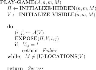
An agent,  , is presented a , is presented a  grid containing grid containing  uniformly distributed mines. The agent’s objective is to expose all the empty grid locations and none of the mines. Information about the mines’ grid locations is gained by exposing empty grid locations which will indicate how many mines exist within a unit (Chebyshev) distance of the grid location. If the exposed grid location is a mine, then the player loses the game. Otherwise, once all empty locations are exposed, the player wins. uniformly distributed mines. The agent’s objective is to expose all the empty grid locations and none of the mines. Information about the mines’ grid locations is gained by exposing empty grid locations which will indicate how many mines exist within a unit (Chebyshev) distance of the grid location. If the exposed grid location is a mine, then the player loses the game. Otherwise, once all empty locations are exposed, the player wins.
|
|
Initialization |
|
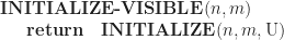
The board consists of hidden and visible states. To represent the hidden,  , and visible state, , and visible state,  , of the board, two character matrices of dimension are used. , of the board, two character matrices of dimension are used.
Characters ‘0’-‘8’ represent the number of neighboring mines, character ‘U’ to represent an unexposed grid location and character ‘*’ for a mine. Neighbors of a grid location |
|
Exposing Cells |
|
|
The expose behavior can be thought of as a flood fill on the grid, exposing any empty region bordered by grid locations containing mine counts and the boundaries of the grid.
A matrix, If a cell location can be exposed, then each of its neighbors will be added to the stack to be inspected. Those neighbors that have already been inspected will be skipped. Once all the reachable grid locations have been inspected, the process terminates. |

|
 is the set of grid locations such that
  . By default,
  .
.

 , represents the topography of the board. A value of zero is reserved for sections of the board that have yet to be visited, a value of one for those that have, two for those that are boundaries and three for mines. A stack,
  , keeps track of locations that should be inspected.
 Verification
Methodology
Statistical tests are used to verify the random aspects of the game’s implementation. I will skip the verification of the game’s logic as it requires use of a number of different methods that are better suited for their own post.
There are two random aspects worth thinking about: the distribution of mines and the distribution of success (i.e., not clicking a mine) for random trials. In both scenarios it made since to conduct Pearson’s chi-squared test. Under this approach there are two hypotheses:
: The distribution of experimental data follows the theoretical distribution
: The distribution experimental data does not follow the theoretical distribution


Mine distribution
The first aspect to verify was that mines were being uniformly placed on the board. For a standard 


In the above experiment, 


Distribution of successful clicks
The second aspect to verify is that the number of random clicks before exposing a mine follows a hypergeometric distribution. The hypergeometric distribution is appropriate since we are sampling (exposing) without replacement (the grid location remains exposed after clicking). This hypothesis relies on a non-flood-fill exposure.
The distribution has four parameters. The first is the number of samples drawn (number of exposures), the second the number of successes in the sample (number of empty exposures), the third the number of successes in the population (empty grid locations) and the last the size of the population (grid locations): 
The expected frequencies for the hypergeometric distribution is given by 


In the above experiment 

Also included in the plot is the observed distribution for a flood based exposure. As one might expect, the observed frequency of more exposures decreases more rapidly than that of the non-flood based exposure.
Agents
Methodology
Much like how a human player would learn to play the game, I decided that each model would have knowledge of game’s mechanics and no prior experience with the game. An alternative class of agents would have prior experience with the game as the case would be in a human player who had studied other player’s strategies.
To evaluate the effectiveness of the models, each played against a series of randomly generated grids and their respective success rates were captured. Each game was played on a standard beginner’s ![[1, 10]](https://s0.wp.com/latex.php?latex=%5B1%2C+10%5D&bg=ffffff&fg=1c1c1c&s=0&c=20201002)
For those models that refer to a probability measure, 
Marginal Model
DevelopmentThe first model to consider is the Marginal Model. It is designed to simulate the behavior of a naive player who believes that if he observes a mine at a grid location that the location should be avoid in future trials. The model treats the visible board,
|

|
 or (a)
  . This model picks the grid location with the greatest empirical probability of being empty:
Test Results
Since the mine distribution is uniform, the model should be equivalent to selecting locations at random. The expected result is that avoiding previously occupied grid locations is an ineffective strategy as the number of mines increases. This does however, provide an indication of what the success rate should look like for chance alone.

Conditional Model
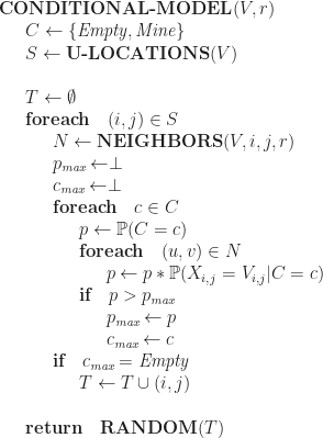
DevelopmentOne improvement over the Marginal Model is to take into account the visual clues made visible when an empty grid location is exposed. Since an empty grid location represents the number of neighboring mines, the Conditional Model can look at these clues to determine whether or not an unexposed grid location contains a mine. This boils down to determining the probability of As in the case of the Marginal Model, the Conditional Model returns the grid location that it has determined has the greatest probability of being empty given its neighbors:
|
|
 . A simplification in calculating the probability is to assume that each piece of evidence is independent. Under this assumption the result is a
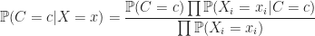
Test Results
The Naïve Bayes Classifier is regarded as being an effective approach to classifying situations for a number of different tasks. In this case, it doesn’t look like it is effective at classifying mines from non-mines. The results are only slightly better than the Marginal Model.

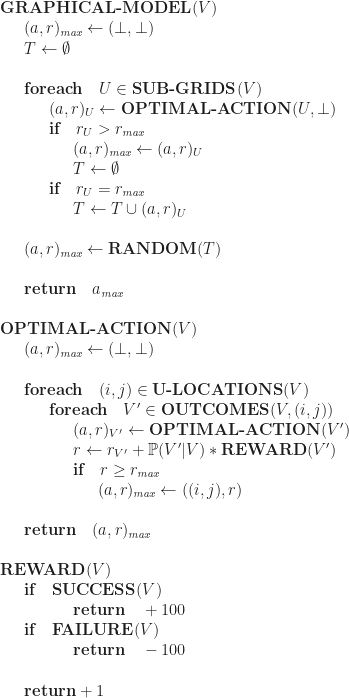
Graphical Model
DevelopmentOne shortfall of the Conditional Model is that it takes a greedy approach in determining which action to take. A more sophisticated approach is to not just consider the next action, but the possible sequence of actions that will minimize the possibility of exposing a mine. Each of the possible observable grids, It is possible to pick a path, Solving for
|
|
 , to the next observable state,
  . Each transition was achieved by performing an action,
  , on the state. The specific action,
  , is chosen from a subset of permitted actions given the state. Each transition has a probability,
  , of taking place.
 , through this graph that minimizes the risk by assigning a reward,
  , to each state and attempting to identify an optimal path,
  , from the present state that yields the greatest aggregate reward,

From the optimal walk, a sequence of optimal actions is determined by mapping
This description constitutes a Markov Decision Process. As is the case for most stochastic processes, it is assumed that the process holds the Markov Property; that future states only depend upon the current states and none of the prior states. In addition to being a Markov Decision Process, this is also an example of Reinforcement Learning.
First thing to observe is that the game state space is astronomical. For a standard beginner’s grid there is at most a sesvigintillion 
To simplify the state space, I chose to only consider 
Test Results
The Graphical Model produces results that are only a margin better than those of the Conditional Model.

Semi-deterministic Model
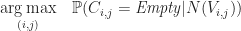
DevelopmentThe last model I’m going to talk about is a semi-deterministic model. It works by using the visible grid to infer the topology of the hidden grid and from the hidden grid, the topology that the visible grid can become. The grid can be viewed as a graph. Each grid location is a vertex and an edge is an unexposed grid location’s influence on another grid location’s neighbor mine count. For each of the exposed grid locations on the board, The model produces its inferred version, For each of the grid locations that are exposed and the inferred influence matches the visible count, then each of the neighbors about that location can be exposed provided they are not already exposed and not an inferred mine. From this set of possibilities, a mine location is chosen. When no mine locations can be determined, then an alternative model can be used. |

|
 , it’s neighbors,
  , are all mines when the number of inbound edges
  , matches the visible mine count
  .
. , of the influence graph
  by using the determined mine locations
 Test Results
Since the model is a more direct attempt at solving the board, its results are superior to the previously presented models. As the number of mines increases, it is more likely that it has to rely on a more probabilistic approach.

Summary
Each of the models evaluated offered incremental improvements over their predecessors. Randomly selecting locations to expose is on par with choosing a location based on previously observed mine locations. The Conditional Model and Graphical Model yield similar results since they both make decisions based on conditioned probabilities. The Semi-deterministic Model stands alone as the only one model that produced reliable results.

The success rate point improvement between the Condition and Marginal models is most notable for boards consisting of three mines and the improvement between Graphical and Semi-deterministic models for seven mines. Improvements between Random and Marginal models is negligible and between Conditional and Graphical is minor for all mine counts fewer than seven.

Given the mathematical complexity and nondeterministic nature of the machine learning approaches, (in addition the the complexity and time involved in implementing those approaches) they don’t seem justified when more deterministic and simpler approaches exist. In particular, it seems like most people have implemented their agents using heuristics and algorithms designed to solve constraint satisfaction problems. Nonetheless, this was a good refresher to some of the elementary aspects of probability, statistics and machine learning.
References
“Classification – Naïve Bayes.” Data Mining Algorithms in R. Wikibooks. 3 Nov. 2010. Web. 30 Oct. 2011.
“Windows Minesweeper.” MinesweeperWiki. 8 Sept. 2011. Web. 30 Oct. 2011.
Kaye, Richard. “Minesweeper Is NP-complete.” [pdf] Mathematical Intelligencer 22.2 (2000): 9-15. Web. 30 Oct. 2011.
Nakov, Preslav, and Zile Wei. “MINESWEEPER, #MINESWEEPER.” 14 May 2003. Web. 14 Apr. 2012.
Richard, Sutton, and Andrew G. Barto. “3.6 Markov Decision Processes.” Reinforcement Learning: An Introduction. Cambridge, Massachusetts: Bradford Book, 1998. 4 Jan. 2005. Web. 30 Oct. 2011.
Rish, Irene “An Empirical Study of the Naive Bayes Classifer.” [pdf] IJCAI-01 Workshop on Empirical Methods in AI (2001). Web. 30 Oct. 2011.
Russell, Stuart J., and Peter Norvig. Artificial Intelligence: A Modern Approach. Upper Saddle River, NJ: Prentice Hall/PearsonEducation., 2003. Print.
Sun, Yijun, and Jian Li. “Adaptive Learning Approach to Landmine Detection.” [pdf] IEEE Transactions of Aerospace and Electronic Systems 41.3 (2005): 1-9. 10 Jan. 2006. Web. 30 Oct. 2011.
Taylor, John R. An introduction to error analysis: the study of uncertainties in physical measurements. Sausalito, CA: University Science Books, 1997. Print.
