Image Processing

Posts Tagged ‘Image Processing’

Category Recognition of Golden and Silver Age Comic Book Covers

Introduction

Motivation

For a while now, I’ve been wanting to work on a computer vision project and decided for my next research focused project that I would learn some image processing and machine learning algorithms in order to build a system that would classify the visual contents of images, a category recognizer. Over the course of the summer I researched several techniques and built the system I had envisioned. The end result is by no means state of the art, but satisfactory for four months of on-and-off development and research. The following post includes my notes on the techniques and algorithms that were used in the project followed by a summary of the system and its performance against a comic book data set that was produced during development.

Subject Matter

The original subject matter of this project were paintings from the 1890s done in the Cloisonnism art style. Artists of the style are exemplified by Emile Bernard, Paul Gaugin and Paul Serusier. The style is characterized by large regions of flat colors outlined by dark lines; characteristics that would be easy to work with using established image processing techniques. During development, it became evident that no one approach would work well with these images. As an alternative, I decided to work with Golden and Silver Age comic book covers from the 1940s to 1960s which also typified this art style. Many of the comic books were drawn by the same individuals such as Jack Kirby, Joe Shuster and Bob Kane. As an added benefit, there are thousands of comic book covers available online compared to the dozens of Cloisonnism paintings.

Representation

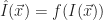
An image is a function, $I : \mathbb{Z}^2 \to \mathbb{Z}^3$ , where each input vector, $\vec{x}$ , represents an image coordinate and each output vector, $\vec{y}$ , represents the red, blue and green (RGB) channels, $\vec{y}_c$ , of an image. Individual input values are bound between zero and the width, $w$ , or height, $h$ , of the image and output values are between zero and $255$ . Each output vector represents a unique color in RGB space giving rise to $2^{24}$ possible colors. Below is a basic sample image broken down into to its individual channels.

From left to right: original image, red channel, blue channel and green channel.
Original image: Action Comics 1 (1938). Art by Joe Shuster. Copyright © 1938 DC Comics, Inc.

Like any other vector field, transformations can be applied to the image to yield a new image, $\hat{I}$ . In image processing, these transformations are referred to as image filters and come in three varieties of point-based, neighbor-based and image-based filters. As the names suggest, point-based filters map single output vectors to a single output vector, neighbor-based filters map neighboring output vectors to a single output vector, and image-based filters map the whole image and a single or neighboring set of output vectors to a single output vector.

There are many different instances of these types of filters, but only those used in this project are discussed below. Computational complexity and efficient algorithms for each type of filter are also discussed where appropriate.

Point-based Filters

Point-based filters, $f : \mathbb{Z}^3 \to \mathbb{Z}^3$ , map an output vector to a new output vector in the form $\hat{I}(\vec{x}) = f(I(\vec{x}))$ . Application of a point-based filter is done in quadratic time with respect to the dimensions of the image $\mathcal{O}(N^2)$ .

Grayscale Projection

It is helpful to collapse the RGB channels of an image down to a single channel for the purpose of simplifying filter results. This can be done by using a filter of the form $f(\vec{y})_c = \frac{ \lVert \vec{y} \rVert_2 }{ \sqrt{3} }$ . Alternatively one can use a filter of the form $f(\vec{y})_c = (0.2126, 0.7152, 0.0722)^T \cdot \vec{y}$ to represent the luminescence of the output vector.

Thresholding

A threshold filter serves as a way to accentuate all values in the image greater than or equal to a threshold, $\gamma$ , or to attenuate all those values less than the threshold.

The first variety is the step threshold filter, 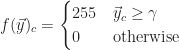$f(\vec{y})_c = \begin{cases} 255 & \vec{y}_{c} \ge \gamma \\ 0 & \text{otherwise} \end{cases}$ , which exhibits an ideal threshold cutoff after the threshold value.

The second variety is a logistic threshold filter, 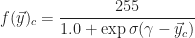$\displaystyle f(\vec{y})_c = \frac{255}{ 1.0 + \exp{\sigma(\gamma - \vec{y}_c)} }$ , with an additional parameter, $\sigma$ , allowing for wiggle room about the threshold yielding a tapered step function as $\sigma$ increases in size.

From left to right: original image, step threshold filter ( $\gamma = 0.5$ ), logistic threshold filter ( $\gamma = 0.5$ , $\sigma = 4$ ), and logistic threshold filter ( $\gamma = 0.5$ , $\sigma = 16$ ).
Original image: The Amazing Spider-Man 1 (1963). Art by Jack Kirby & Steve Ditko. Copyright © 1963 Non-Pareil Publishing Corp.

Neighbor-based Filters

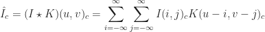
All neighbor-based filters take the output vectors neighboring an input vector to calculate a new output vector value. How the neighboring output vectors should be aggregated together is given by a kernel image, $K$ , and the computation is represented as a two-dimensional, discrete convolution.

$\hat{I}_c = \displaystyle (I \star K)(u,v)_c = \sum_{i=-\infty}^{\infty} \sum_{j=-\infty}^{\infty} I(i,j)_c K(u-i,v-j)_c$

Neighbor-based filters can be applied naïvely in quartic time as a function of the image and kernel dimensions, $\mathcal{O}(N^4)$ . However, a more efficient implementation allows for $\mathcal{O}(N^2 \log_2 N)$ time by way of the Discrete Fourier Transform.

$\displaystyle \mathcal{F}(f)(x) = \sum_{n=0}^{N-1} f(n) \exp{ -2 \pi i \frac{n}{N} x}$

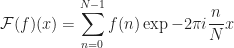
The Discrete Fourier Transform is a way of converting a signal residing in the spatial domain into a signal in the frequency domain by aggregating waveforms of varying frequencies where each waveform is amplified by its corresponding value in the input signal. The Inverse Discrete Fourier Transform maps a frequency domain signal back to the spatial domain.

$\displaystyle \mathcal{F}^{-}(f)(x) = \frac{1}{N} \sum_{n=0}^{N-1} f(n) \exp{ 2 \pi i \frac{n}{N} x}$

Applying the Discrete Fourier Transform to a convolution, $\mathcal{F}(f \star g)$ , comes with the convenient property that the transformed convolution can be rewritten as the product of the transformed functions, $\mathcal{F}(f) \mathcal{F}(g)$ , by way of the Convolution Theorem.

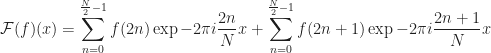
The improved time complexity is achieved by using a divide a conquer algorithm known as the Fast Fourier Transform which takes advantage of the Danielson-Lanczos Lemma which states that the Discrete Fourier Transform of a signal can be calculated by splitting the signal into two equal sized signals and computing their Discrete Fourier Transform.

$\displaystyle \mathcal{F}(f)(x) = \sum_{n=0}^{\frac{N}{2} - 1} f(2n) \exp{ -2 \pi i \frac{2n}{N} x} + \sum_{n=0}^{\frac{N}{2} - 1} f(2n+1) \exp{ -2 \pi i \frac{2n+1}{N} x }$

$\displaystyle \mathcal{F}(f)(x) = \sum_{n=0}^{\frac{N}{2} - 1} f(2n) \exp{ -2 \pi i \frac{n}{N / 2} x} + \exp{ -2 \pi i \frac{x}{N} } \sum_{n=0}^{\frac{N}{2} - 1} f(2n+1) \exp{ -2 \pi i \frac{n}{ N / 2 } x }$

$\displaystyle \mathcal{F}(f)(x) = \mathcal{F}(f_{even})(x) + \mathcal{F}(f_{odd})(x) \exp{ -2 \pi i \frac{x}{N} }$

For the purposes of image processing, we use the two-dimensional Discrete and Inverse Discrete Fourier Transform.

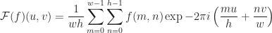
$\displaystyle \mathcal{F}(f)(u, v) = \frac{1}{w h} \sum_{m = 0}^{w - 1} \sum_{n = 0}^{h-1} f(m,n) \exp{-2 \pi i \left (\frac{m u}{h} + \frac{nv}{w} \right) }$

The expression can be rearranged to be the Discrete Fourier Transform of each column in the image and then computing the resulting Discrete Fourier Transform of those results to obtain the full two-dimensional Discrete Fourier Transform.

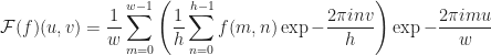
$\displaystyle \mathcal{F}(f)(u, v) = \frac{1}{w} \sum_{m = 0}^{w-1} \left ( \frac{1}{h} \sum_{n = 0}^{h-1} f(m,n) \exp{-\frac{2 \pi i n v}{h}} \right) \exp{-\frac{2 \pi i m u}{w}}$

As a result, we can extend the Fast Fourier Transform in one dimension easily into two dimensions producing a much more efficient time complexity.

Weighted Means: Gaussian and Inverse Distance

Weighted mean filters are used to modify the morphology of an image by averaging neighboring output vectors together according to some scheme.

A Gaussian filter is used to blur an image by using the Gaussian distribution with standard deviation, $\sigma$ , as a kernel.

$\displaystyle K(u, v)_c = \frac{1}{2 \pi \sigma^2} \exp{-\frac{u^2+v^2}{2 \sigma^2} }$

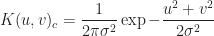
The inverse distance filter calculates how far the neighboring output vectors are with respect to the new output vector being calculated. Each result is also scaled by the parameter, $\gamma$ , allowing for contrast adjustments.

$\displaystyle K(u, v)_c = \begin{cases} \gamma \lVert (u-i, v-j) \rVert^{-} & (u,v) \neq (i,j) \\ 0 & \text{otherwise} \end{cases}$

Laplacian

A Laplacian filter detects changes in an image and can be used for sharpening and edge detection. Much like in calculus of a single variable, the slope of a surface can be calculated by the Gradient operator, $\displaystyle \nabla = \left ( \frac{\partial}{\partial x}, \frac{\partial}{\partial y} \right )$ . Since it is easier to work with a scalar than a vector, the magnitude of the gradient is given by the Laplacian operator, $\displaystyle \Delta = \nabla \cdot \nabla = \frac{\partial^2}{\partial x^2} + \frac{\partial^2}{\partial y^2}$ .

Since an image is a discrete function, the Laplacian operator needs to be approximated numerically using a central difference. $h$ represents the spacing between successive samples of the underlying function. Since the finest resolution that can be achieved in an image is an individual displacement, $h = 1$ .

$\displaystyle \Delta I \approx \frac{I(x + h, y) + I(x, y + h) - 4 I(x,y) - I(x - h, y) + I(x, y - h)}{h^2}$

$\displaystyle \Delta I \approx I \star K = I \star \frac{1}{h^2} \begin{pmatrix} 0 & 1 & 0 \\ 1 & -4 & 1 \\ 0 & 1 & 0 \end{pmatrix}$

From left to right: original image, Gaussian filter ( $\sigma = 4.0$ ), inverse distance filter ( $\gamma = 2.0$ ) and Laplacian filter.
Original image: Batman 1 (1940). Art by Bob Kane. Copyright © 1940 DC Comics, Inc.

Image-based Filters

Image-based filters calculate some information about the contents of the image and then use that information to generate the appropriate point-based and neighbor based filters.

Normalization

The normalization process computes the minimum, $\vec{y}_{c}^{\text{min}}$ and maximum, $\vec{y}_{c}^{\text{max}}$ values of each channel and linearly maps all values between those extrema to new values between the possible channel extrema of $c^{\text{min}} = 0$ and $c^{\text{max}} = 255$ .

$\displaystyle \hat{I}(\vec{x})_c = \frac{I(\vec{x})_c - \vec{y}^{\text{min}}_c}{\vec{y}^{\text{max}}_c - \vec{y}^{\text{max}}_c} (c^\text{max} - c^\text{min}) + c^\text{min}$

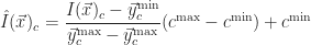
This particular image-based filter can be applied in quadratic time, $\mathcal{O}(N^2)$ , to calculate the extrema of the image and apply the linear map.

From left to right: original image, normalized image and accompanying histograms.
Original image: Daredevil 1 (1964). Art by Jack Kirby. Copyright © 1964 Marvel Comics.

Edge Detection

Edge detection is the process of identifying changes (e.g., texture, color, luminance and so on) in an image. As alluded to in the image processing section, the Laplacian filter is central to detecting edges within an image. As a result A sequence of filters is used before and after a Laplacian filter to produce a detector that consistently segments comic book covers. The following sequence of filters was used.

Grayscale Projection – Since all logical components of a comic book cover are separated by inked lines, it is permissible to ignore the full set of RGB channel information and collapse the image down to a grayscale image.
Normalization – It is conceivable that the input image has poor contrast and brightness. To ensure that the full range of luminescence values are presented, the image is normalized.
Gaussian ( $\sigma = 1.5$ ) – An image may have some degree of noise superimposed on the image. To reduce the noise, the image is blurred using a Gaussian filter with a standard deviation of $1.5$ . This is enough to smooth out the image without distorting finer image detail.
Laplacian – Once the image has been prepared, its edges are calculated using the Laplacian filter.
Normalization – Most of the changes in the image may be subtle and need to make sure that all edge information is accentuated as much as possible by applying a normalization filter.
Step Threshold ( $\gamma = 0.05$ ) – Since a partial edge isn’t particularly useful information, any edge RGB value less than $12.75$ is attenuated to zero and all other values accentuated to $255$ .
Inverse Distance ( $\gamma = 1.5$ ) – It is possible that during the threshold process that discontinuities were introduced into some of the edges. To mitigate this impact, an inverse distance filter is used to inflate existing edges and intensify the result with a gain of $1.5$ .

From left to right, top to bottom: original image, grayscale projection, normalization, Gaussian ( $\sigma = 1.5$ ), Laplacian, normalization, step threshold ( $\gamma = 0.05$ ), inverse distance ( $\gamma = 1.5$ ).
Original image: Captain America 111 (1964). Art by Jim Steranko. Copyright © 1968 Marvel Comics.

The complete edge detection process takes computational complexity of $\mathcal{O}(N^2 \log_2 N)$ due to the neighbor-based filters used to eliminate noise and smooth edge discontinuities.

Segmentation

With the edge image it is possible to segment the image into its visual components. This is achieved by doing a flood fill on the image and using the edge image as the boundaries for the fill. Once the fill runs out of points to flood, the segment is complete and the next remaining point in the image is considered. To reduce the number of minuscule segments, only those segments representing $0.1 \%$ of the image are included.

From left to right: original image, edge image, sample overlaid segments and sample segments.
Original image: Fantastic Four Vol 1 59 (1967). Art by Jack Kirby. Copyright © 1967 Marvel Comics.

Machine Learning

Classifiers

The task of classification is to identify decision boundaries separating all of the classification within the data set. Such data sets can be linearly or non-linearly separable and as a result, classifiers were developed to solve the linear case and then adapted to deal with the more complicated non-linear case. While there are a number of classifiers, only the K-Nearest Neighbor and Support Vector Machine classifiers were researched and implemented in this project.

K-Nearest Neighbor

The K-Nearest Neighbor classifier is an online classifier which operates under the assumption that a yet to be classified vector is most likely to be the same classification as those $k$ training vectors which are closest to the vector based on a distance measure, $d : \mathbb{R}^n \times \mathbb{R}^n \to \mathbb{R}$ .

Distance can be measured in a variety of ways for arbitrary vectors, $\vec{x}, \vec{y} \in \mathbb{R}^n$ , residing in some real space. The most common of which are specialized cases of the Minkowski distance.

$\displaystyle d_{p}(\vec{x},\vec{y}) = \left ( \sum_{i = 0}^{n} \lvert \vec{x}_{i} - \vec{y}_{i} \rvert^{p} \right )^{ \frac{1}{p} }$

The Manhattan distance, $d_{1}(\vec{x},\vec{y})$ , yields the distance traveled along a grid between two vectors (hence a name in reference to the New York City borough). The Euclidean distance, $d_{2}(\vec{x}, \vec{y})$ , gives the distance between the vectors in the usual familiar sense. The last specialized cased considered is the Chebyshev distance, $d_{\infty}(\vec{x},\vec{y})$ , which gives the maximum distance between any one dimension of the two vectors.

Two factors affect the efficacy of the algorithm. The first is the dimension of the data, $n$ , and the size of the train data set, $N$ . As the training data set increases with size, there are more vectors which a test vector must be compared against. As a result, an efficient means of searching the training set must be used to yield satisfactory performance. This can be achieved by using kd-Trees which give $\mathcal{O}(\log N)$ search performance or branch and bound methods giving similar performance. As the dimensionality of the dataset increases, the efficacy of kd-Trees diminishes to a near linear search of the training data set due to the “curse of dimensionality.”

From left to right: Test point (green triangle) near two categorizes, identification of nearest neighbors, and resolved category.

Support Vector Machine

Formulation

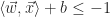
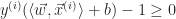
The Support Vector Machine classifier is an offline linear, binary classifier which operates under the assumption that a training set, $(\vec{x}, y)^{(i)} \in \mathcal{D}$ , consists of linearly separable classifications, $y \in \lbrace -1, +1 \rbrace$ , of data, $\vec{x} \in \mathbb{R}^n$ , by some optimal hyperplane of the form $\langle \vec{w}, \vec{x} \rangle + b = 0$ . Where $\langle \cdot, \cdot \rangle$ is the inner product, $\vec{w} \in \mathbb{R}^n$ and $b \in \mathbb{R}$ . When $\langle \vec{w}, \vec{x} \rangle + b \ge 1$ , then the classification $+1$ is presented and when $\langle \vec{w}, \vec{x} \rangle + b \le -1$ , the classification $-1$ is presented.

From left to right: Training data of two categorizes, optimally separating hyperplane, and resolved categorizes in $\mathbb{R}^2$ .

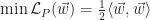
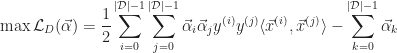
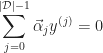
The hyperplane is padded by two hyperplanes separated by an equal distance to the nearest training examples of each classification. The span between the supporting hyper planes is the margin. The goal then is to pick a hyperplane which provides the largest margin between the two separable classifications. The margin between the supporting hyperplanes is given by $\displaystyle \frac{2}{\lVert \vec{w} \rVert}$ . Given the demarcation criteria, the maximum margin will also be subject to the constraint that all training examples satisfy $y^{(i)} (\langle \vec{w}, \vec{x}^{(i)} \rangle + b) - 1 \ge 0$ . As a result of the objective function and accompanying linear constraint, the problem is stated in terms of its native primal Quadratic Programming form.

$\min \mathcal{L}_P(\vec{w}) = \frac{1}{2} \langle \vec{w}, \vec{w} \rangle$ subject to $y^{(i)} (\langle \vec{w}, \vec{x}^{(i)} \rangle + b) - 1 \ge 0$ $\forall (\vec{x}, y)^{(i)} \in \mathcal{D}$

To find the optimal parameters, it is easier to translate the problem into a dual form by applying the technique of Lagrange Multipliers. The technique takes an objective function, $f$ , and constraint functions, $g^{(i)}$ , and yields a new function $\mathcal{L}(\vec{x}, \vec{\alpha}) = f(\vec{x}) + \sum \vec{\alpha}_i g(\vec{x})^{(i)}$ to be optimized subject to the added constraint $\vec{\alpha}_i \ge 0$ $\forall i$ .

$\displaystyle \max_{\vec{\alpha}} \mathcal{L}(\vec{w}, b, \vec{\alpha}) = \frac{1}{2} \langle \vec{w}, \vec{w} \rangle - \sum_{i=0}^{\lvert \mathcal{D} \rvert-1} \vec{\alpha}_{i} (y^{(i)} (\langle \vec{w}, \vec{x}^{(i)} \rangle + b) - 1)$ $\vec{\alpha} \in \mathbb{R}^{\lvert \mathcal{D} \rvert }$ subject to $\vec{\alpha}_{i} \ge 0$ $\forall i$

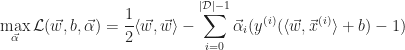
The next step is to differentiate the objective function with respect to the parameters to determine the optimal solution. Since the function is concave, the results will yield the desired maximum constraints.

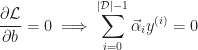
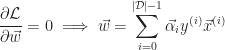
$\displaystyle \frac{\partial \mathcal{L}}{\partial b} = 0 \implies \sum_{i=0}^{\lvert \mathcal{D} \rvert-1} \vec{\alpha}_i y^{(i)} = 0$ $\displaystyle \frac{\partial \mathcal{L}}{\partial \vec{w}} = 0 \implies \vec{w} = \sum_{i=0}^{\lvert \mathcal{D} \rvert-1} \vec{\alpha}_i y^{(i)} \vec{x}^{(i)}$

As a result the dual problem can be written as the following:

$\displaystyle \max \mathcal{L}_D(\vec{\alpha}) = \frac{1}{2} \sum_{i=0}^{\lvert \mathcal{D} \rvert-1} \sum_{j=0}^{\lvert \mathcal{D} \rvert-1} \vec{\alpha}_i \vec{\alpha}_j y^{(i)} y^{(j)} \langle \vec{x}^{(i)}, \vec{x}^{(j)} \rangle - \sum_{k=0}^{\lvert \mathcal{D} \rvert-1} \vec{\alpha}_k$ subject to $\vec{\alpha}_{i} \ge 0$ $\forall i$ , $\displaystyle \sum_{j=0}^{\lvert \mathcal{D} \rvert-1} \vec{\alpha}_j y^{(j)} = 0$

Handling of non-linearly separable data

In the event that the data is not linearly separable, then an additional parameter, $C$ , is added as a penalty factor for those values that reside on the wrong side of the hyperplane. The derivation for the quadratic program is identical to the one presented above with the exception that the lagrange multipliers now have an upper boundary $0 \le \vec{\alpha}_i \le C$ $\forall i$ .

Non-linear classification

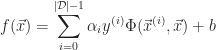
By way of Mercer’s Theorem, the linear Support Vector Machine can be modified to allow for non-linear classification through the introduction of symmetric, positive semidefinite kernel functions, $\Phi : \mathbb{R}^n \times \mathbb{R}^n \to \mathbb{R}$ . The idea being that if the data is not linearly separable in its present dimensional space that by mapping it to a higher dimensional space that the data may become linearly separable by some higher dimensional hyperplane. The benefit of a kernel function is that the higher dimensional vector need not be computed explicitly. This “kernel trick” allows for all inner products in the dual representation to be substituted with a kernel.

$\displaystyle \max \mathcal{L}_D(\vec{\alpha}) = \frac{1}{2} \sum_{i=0}^{\lvert \mathcal{D} \rvert-1} \sum_{j=0}^{\lvert \mathcal{D} \rvert-1} \vec{\alpha}_i \vec{\alpha}_j y^{(i)} y^{(j)} \Phi(\vec{x}^{(i)}, \vec{x}^{(j)}) - \sum_{k=0}^{\lvert \mathcal{D} \rvert-1} \vec{\alpha}_k$ subject to $0 \le \vec{\alpha}_{i} \le C$ $\forall i$ , $\displaystyle \sum_{j=0}^{\lvert \mathcal{D} \rvert-1} \vec{\alpha}_j y^{(j)} = 0$

And the decision hyperplane function then becomes:

$\displaystyle f(\vec{x}) = \sum_{i=0}^{\lvert \mathcal{D} \rvert-1} \alpha_i y^{(i)} \Phi (\vec{x}^{(i)}, \vec{x}) + b$

The following are some typical kernels:

Linear – $\Phi(\vec{x}, \vec{y}) = \langle \vec{x}, \vec{y} \rangle$
Polynomial – $\Phi(\vec{x}, \vec{y}) = (\gamma \langle \vec{x}, \vec{y} \rangle + r)^d$ $\gamma > 0$
Radial basis function – $\Phi(\vec{x}, \vec{y}) = \exp{-\gamma \langle \vec{x} - \vec{y}, \vec{x} - \vec{y} \rangle}$ $\gamma > 0$
Sigmoid – $\Phi(\vec{x}, \vec{y}) = \tanh (\gamma \langle \vec{x}, \vec{y} \rangle + r)$

From a practical point of view, only the linear and radial basis function kernels from this list should be considered since the polynomial kernel has too many parameters to optimize and the sigmoid kernel does not satisfy the positive semidefinite kernel matrix requirement of Mercer’s Theorem.

Algorithmic details

The Support Vector Machine classifier can be implemented using a quadratic programming solver or by incremental descent algorithms. Both methods work, but are difficult to implement and expensive to procure. An alternative is the Sequential Minimal Optimization algorithm developed by John Platt at Microsoft Research. The algorithm works by analytically solving the dual problem for the case of two training examples then iterating over all of the lagrange multipliers verifying that the constraints are satisfied. For those that are not, the algorithm computes new lagrange multiplier values. The full details of the algorithm can be found in Platt’s paper.

The time complexity of the algorithm is quadratic with respect to the number of training samples and support vectors $\mathcal{O}(N^2)$ .

The time complexity of evaluating the decision function is linear with respect to the number of support vectors $\mathcal{O}(N)$ .

Multiclass Classification

The classification methods presented in the previous section are utilized as binary classifiers. These classifiers can be used to classify multiple classifications by employing a one-vs-all or all-vs-all approach. In the former a single classification is separated from the remaining classifications to produce $N$ classifiers for the $N$ classifications. Each classifier is then used to evaluate a vector and the classifier with the highest confidence is then used to declare the classification.

In the latter, a single classification is compared individually to each other classification resulting in $\frac{N(N - 1)}{2}$ classifiers. All of the classifiers are then evaluated against the test vector and the classification with the greatest consensus from the classifiers is declared the classification of the test vector.

Both methods have their place. The benefit of a one-vs-all approach is that there are fewer classifiers to maintain. However, training a single classifier on a complete data set is time consuming and can give deceptive performance measures. All-vs-all does result in more classifiers, but it also provides for faster training which can be easily parallelized on a single machine and distributed to machines on a network.

Classifier Evaluation

Individual classifiers are evaluated by training the classifier against a data set and then determining how many correct and incorrect classifications were produced. This evaluation produces a confusion matrix.

Confusion matrix defintion and associated terms.
		Predicted Classification
		Positive	Negatives	Total
Actual Classification	Positive	(TP) True Positive	(FN) False Negative	(AP) Actual Positives
Actual Classification	Negatives	(FP) False Positive	(TN) True Negative	(AN) Actual Negatives
	Total	(PP) Predicted Positives	(PN) Predicted Negatives	(N) Examples

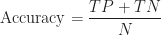
The confusion matrix is used to calculate a number of values which are used to evaluate the performance of the classifier. The first of which is the accuracy and error of the classifier. Accuracy measures the number of instances where the actual and predicted classifications matched up and the error for when they do not.

$\displaystyle \text{Accuracy} = \frac{TP + TN}{N}$ $\displaystyle \text{Error} = \frac{FP + FN}{N}$

Since we should expect to get different results each time we evaluate a classifier, the values that we obtain above are sample estimates of the true values that are expected. Given enough trails and measurements, it is possible to determine empirically what the true values actually are. However, this is time consuming and it is instead easier to use confidence intervals to determine what interval of values a measurement is mostly likely to fall into.

Training and Testing

Each of the classifiers presented have some number of parameters that must be determined. The parameters can be selected by having some prior knowledge or by exploring the parameter space and determining which parameters yield optimal performance. This is done by performing a simple grid search over the parameter space and evaluating and attempting to minimize the error.

K-folds cross-validation is used at each grid location to produce a reliable measure of the error. The idea is that a data set is split into $k$ disjoint sets. The first set is used as a validation set and the remaining $k - 1$ sets are used in unison as the training data set for the classifier. This process is done on the next set and so on until all $k$ sets have been used as a validation set.

System

Implementation

The system was implemented in C# 4.0 on top of the Microsoft .NET Framework. The user interface was written by hand using the WinForms library. No other third-party libraries or frameworks were used. When possible, all algorithms were parallelized to take advantage of multi-core capabilities to improve processing times.

Summary

The system consists of two modes of operation: training and production. In training, a human classifier labels image segments with an appropriate classification. New image segments are then taken into consideration during the training of machine learning algorithms. Those algorithms producing the lowest error for a given classification are then used in production mode. During production, a user submits an image and each image segment is then evaluated against the available classifiers. Those image segments are then presented to the user with the most likely classification. These two modes along with their workflows and components are illustrated in the following diagram.

System inputs, components and outputs used for training and production workflows.

Training Mode

Data Set Construction

The user interface of the system allows users to add an image segment to a local data set of images. Once added, the image is then processed to yield image segments. The user can then label an image segment by editing the segment and moving on to the next image segment. This allows for easy and efficient human classification of data. If the user does not wish to keep the image, he or she may remove the image from the data set as well.

Data set construction tab.
Input image: Superman 14 (1942). Art by Fred Ray. Copyright © 1942 DC Comics, Inc.

Data Set Cleaning

During the construction phase, errors may be introduced into the data set typically in the case of typos or forgetting which segment was currently being edited. The data set is cleaned by listing out all available classifications and presenting the user with all available segments associated with that classification. The user can then review the image segment as it was identified in the source image. If the user does not wish to keep the classification, he or she may remove the image from the data set as well.

Data set cleaning tab.
Input image: Action Comics 62 (1943). Art by Jack Burnley. Copyright © 1943 DC Comics, Inc.

Data Set Statistics

The data set consists of 496 comic book covers pulled from the Cover Browser database of comic book covers. The first 62 consecutive published comic book covers where used from Action Comics, Amazing Spider-man, Batman, Captain America, Daredevil, Detective Comics, Superman, and Wonder Woman and then processed by the image processing subsystem yielding 24,369 image segments. 11,463 of these segments represented classifiable segments which were then labeled by hand over the course of two weeks; the remaining segments were then discarded.

Data Set Distribution consists of predominately clothing and text with equal representation from all comic book series sources.

In total, there were 239 classifications identified in the data set among 18 categories. Text, clothing, geography, and transportation categories accounting for 90% of the data set. Since the majority of classification were incidental, only those classifications having 50 or more image segments were considered by the application leaving a total of 38 classifications.

Classifier Evaluation

For the 38 classifications meeting the minimum criteria for classification, the K-Nearest Neighbor approach worked well in distinguishing between text classifications from other classifications and between intra-text classifications for both all-vs-all and one-vs-all schemes.


All-vs-All K-Nearest Neighbor Performance.	One-vs-All K-Nearest Neighbor Performance.

The Support Vector Machine approach presented unremarkable results for both all-vs-all and one-vs-all methods. In the former, only a few pairings resulted in acceptable error rates whereas the later presented only a couple acceptable error rates.


All-vs-All Support Vector Machine Performance.	One-vs-All Support Vector Machine Performance.

For both classification methods presented, the all-vs-all method yielded superior results to the one-vs-all method. In comparing the two classifier methods, the K-Nearest Neighbor seems to have done better than the Support Vector Machine approach, contrary to what was expected from literature. Both classifier methods are used in production mode.

Production Mode

Production mode allows the end user to add an image to the data set and then review the most likely classifications produced by evaluating each image segment against the available set of classifiers. The end user is then expected to review each segment and accept or reject the suggested classification. Aside from this additional functionality, production mode is nearly identical in functionality to training mode.

Production data set construction tab.
Input image: Detective Comics 36 (1940). Art by Bob Kane. Copyright © 1940 DC Comics, Inc.

Conclusions

The time spent on this project was well spent. I met the objectives that I laid out at the beginning of the project and now have a better understanding of the image processing algorithms and machine learning concepts from a theoretical and practical point of view.

Future Work

Segmentation

One issue with the existing implementation is that it over segments the image. Ideally, fewer segments would be produced that are more closely aligned with their conceptual classification. There are a number of popular alternatives to the approach taken, such as level set methods, which should be further investigated.

Classification

The approach taken to map scaled versions of the image segments to a $2^{10}$ space is simple to implement, but it did not assist well in the classification process. Alternative mappings such as histogram models should be evaluated in the future to decrease classification times and to determine if classification error rates can be reduced.

System User Interface

While it was disappointing to have spent so much time building a data set only to have to limit what was considered, it assisted me in building a user interface that had to be easy and fast to use. The application can certainly be developed further and adapted to allow for other data sets to be constructed, image segmentation methods to be added and additional classifications to be evaluated.

System Scalability

The system is limited now to a single machine, but to grow and handle more classifications, it would need to be modified to run on multiple machines, have a web-based user interface developed and a capable database to handle the massive amounts of data that would be required to support a data set on the scale of the complete Cover Browser’s or similar sites’ databases (e.g., 450,000 comic book covers scaled linearly would require 546 GiB of storage.) Not to mention data center considerations for overall system availability and scalability.

References

Aly, Mohamed. Survey on Multiclass Classification Methods. [pdf] Rep. Oct. 2011. Caltech. 24 Aug. 2012.

Asmar, Nakhle H. Partial Differential Equations: With Fourier Series and Boundary Value Problems. 2nd ed. Upper Saddle River, NJ: Pearson Prentice Hall, 2004. Print.

Bousquet, Olivier, Stephane Boucheron, and Gabor Lugosi. “Introduction to Statistical Learning Theory.” [pdf] Advanced Lectures on Machine Learning 2003,Advanced Lectures on Machine Learning: ML Summer Schools 2003, Canberra, Australia, February 2-14, 2003, Tübingen, Germany, August 4-16, 2003 (2004): 169-207. 7 July 2012.

Boyd, Stephen, and Lieven Vandenberghe. Convex Optimization [pdf]. N.p.: Cambridge UP, 2004. Web. 28 June 2012.

Burden, Richard L., and J. Douglas. Faires. Numerical Analysis. 8th ed. Belmont, CA: Thomson Brooks/Cole, 2005. Print.

Caruana, Rich, Nikos Karampatziakis, and Ainur Yessenalina. “An Empirical Evaluation of Supervised Learning in High Dimensions.” [pdf] ICML ’08 Proceedings of the 25th international conference on Machine learning (2008): 96-103. 2 May 2008. 6 June 2012.

Fukunaga, Keinosuke, and Patrenahalli M. Narendra. “A Branch and Bound Algorithm for Computing k-Nearest Neighbors.” [pdf] IEEE Transactions on Computers (1975): 750-53. 9 Jan. 2004. 27 Aug. 2012.

Gerlach, U. H. Linear Mathematics in Infinite Dimensions: Signals, Boundary Value Problems and Special Functions. Beta ed. 09 Dec. 2010. Web. 29 June 2012.

Glynn, Earl F. “Fourier Analysis and Image Processing.” [pdf] Lecture. Bioinformatics Weekly Seminar. 14 Feb. 2007. Web. 29 May 2012.

Gunn, Steve R. “Support Vector Machines for Classification and Regression” [pdf]. Working paper. 10 May 1998. University of Southampton. 6 June 2012.

Hlavac, Vaclav. “Fourier Transform, in 1D and in 2D.” [pdf] Lecture. Czech Technical University in Prague, 6 Mar. 2012. Web. 30 May 2012.

Hsu, Chih-Wei, Chih-Chung Chang, and Chih-Jen Lin. A Practical Guide to Support Vector Classification. [pdf] Tech. 18 May 2010. National Taiwan University. 6 June 2012.

Kibriya, Ashraf M. and Eibe Frank. “An empirical comparison of exact nearest neighbour algorithms.” [pdf] Proc 11th European Conference on Principles and Practice of Knowledge Discovery in Databases. (2007): 140-51. 27 Aug. 2012.

Marshall, A. D. “Vision Systems.” Vision Systems. Web. 29 May 2012.

Panigraphy, Rina. Nearest Neighbor Search using Kd-trees. [pdf] Tech. 4 Dec. 2006. Stanford University. 27 Aug. 2012.

Pantic, Maja. “Lecture 11-12: Evaluating Hypotheses.” [pdf] Imperial College London. 27 Aug. 2012.

Platt, John C. “Fast Training of Support Vector Machines Using Sequential Minimal Optimization.” [pdf] Advances in Kernel Methods – Support Vector Learning (1999): 185-208. Microsoft Research. Web. 29 June 2012.

Sonka, Milan, Vaclav Hlavac, and Roger Boyle. Image Processing, Analysis, and Machine Vision. 2nd ed. CL-Engineering, 1998. 21 Aug. 2000. Web. 29 May 2012.

Szeliski, Richard. Computer vision: Algorithms and applications. London: Springer, 2011. Print.

Tam, Pang-Ning, Michael Steinbach, and Vipin Kumar. “Classification: Basic Concepts, Decision Trees, and Model Evaluation.” [pdf] Introduction to Data Mining. Addison-Wesley, 2005. 145-205. 24 Aug. 2012.

Vajda, Steven. Mathematical programming. Mineola, NY: Dover Publications, 2009. Print.

Welling, Max. “Support Vector Machines“. [pdf] 27 Jan. 2005. University of Toronto. 28 June 2012

Weston, Jason. “Support Vector Machine (and Statistical Learning Theory) Tutorial.” [pdf] Columbia University, New York City. 7 Nov. 2007. 28 June 2012.

Zhang, Hui, Jason E. Fritts, and Sally A. Goldman. “Image Segmentation Evaluation: A Survey of Unsupervised Methods.” [pdf] Computer Vision and Image Understanding 110 (2008): 260-80. 24 Aug. 2012.

Copyright

Images in this post are used under §107(2) Limitations on exclusive rights: Fair use of Chapter 1: Subject Matter and Scope of Copyright of the of the Copyright Act of 1976 of Title 17 of the United States Code.

Written by lewellen

2012-10-01 at 8:00 am

Posted in Algorithms, Artificial Intelligence, Computer Graphics

Tagged with Category Recognition, Computer Vision, Edge Detection, Fast Fourier Transform, FFT, Image Processing, Image Segmentation, K-Folds Cross-validation, K-Nearest Neighbors, KNN, Quadratic Programming, Sequential Minimal Optimization, SMO, Support Vector Machine, SVM