Algorithms for Procedurally Generated Environments

Fig. 1: Demonstration of different graphics techniques and features of the procedurally generated environment.

Introduction

I recently completed a graduate course in Computer Graphics that required us to demonstrate a significant understanding of OpenGL and general graphics techniques. Given the short amount of time to work with, I chose to work on creating a procedurally generated environment consisting of land, water, trees, a cabin, smoke, and flying insects. The following write-up explains my approach and the established algorithms that were used to create the different visual effects showcased in the video above.

Terrain

Fig. 2: First few iterations of the Midpoint Displacement algorithm.

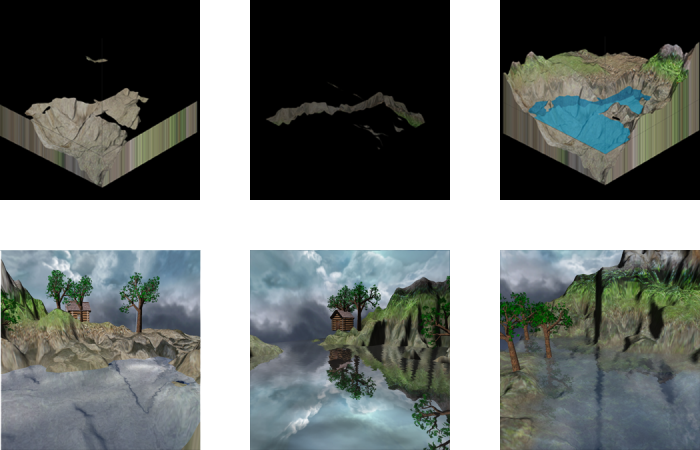
There are a variety of different techniques for creating terrain. More complex ones rely on visualizing a three dimensional scalar field, while simpler ones visualize a two dimensional surface defined by a fixed image, or dynamically using a series of specially crafted functions or random behavior. I chose to take a fractal-based approach given by [FFC82]’s Midpoint Displacement algorithm. A two dimensional grid of size (for ) is allocated with each entry representing the height of the terrain at that row and column position. Beginning with the corners, the corresponding four midpoints, as well as singular center, are found and their height calculated by drawing from a uniform random variable whose support is given by the respective corners. The newly assigned values now form four separate squares which can be assigned values recursively as shown above. The Midpoint Displacement algorithm produces noisy surfaces that are jagged in appearance. To smooth out the results, a Gaussian Filter is applied to the surface twice in order to produce a more natural, smooth looking surface.

Face normals can be found by taking the cross product of the forward differences in both the row and column directions, however this leads to a faceted looking surface. For a more natural appearance, vertex normals are calculated using central differences in the row and column direction. The cross product of these approximations then gives the approximate surface normal at each vertex to ensure proper lighting.

Fig. 3: Example process of blending an elevation band texture with the base texture to create geographically correct looking terrain textures.

Texturing of the terrain is done by dynamically blending eight separate textures together based on terrain height as shown above. The process begins by loading in a base texture which is applied to all heights of the terrain. The next texture to apply is loaded, and an alpha mask is created and applied to the next texture based on random noise and a specific terrain height band. Blending of the masked texture and base texture is a function of the terrain’s height where the normalized height is passed through a logistic function to decide what portion of each texture should be used. The combined texture then serves as a new base texture and the process repeats until all textures have been blended together.

Water

In order to generate realistic looking water, a number of different OpenGL abilities were employed to accurately capture a half dozen different water effects consisting of reflections, waves, ripples, lighting, and Fresnel effects. Compared to other elements of the project, water required the largest graphics effort to get right.

Fig. 4: The different rendering passes for creating realistic looking water with reflections and refraction.

To obtain reflections, a three-pass rendering process is used. In the first pass, the scene is clipped and rendered to a frame buffer (with color and depth attachments) from above the water revealing only what is below the surface for the refraction effects. The second pass clips and renders the scene to a frame buffer (with only a color attachment) from below the water surface revealing only what is above the water for the reflection effects. The third pass then combines these buffers on the water surface through vertex and fragment shaders to give the desired appearance. To map the frame buffer renderings to the water surface, the clipped coordinates calculated in the vertex shader are converted to normalized device coordinates through perspective division in the fragment shader which allows one to map the coordinate of the texture as it should appear on the screen to coordinates of the water surface.

Fig. 5: Reflection, ripples normal map, water depth, refraction, specular normal map, and depth buffer textures used to achieve different visual effects.

To create the appearance of water ripples, a normal map is sampled and the resulting time varying displacement is used to sample the reflection texture for the fragment’s reflection color. Next, a similar sampling of the normal map is done at a coarser level to emulate the specular lighting that would appear on the subtle water waves created by the vertex shader. Refraction ripples and caustic lighting are achieved by sampling from the normal map just as the surface ripples and specular lighting were. To make the water appear cloudy, the depth buffer from the refraction rendering is used in conjunction with water depth so that terrain deeper under water is less visible as it would be in real life.

To combine the reflection and refraction components, the Fresnel Effect is used. This effect causes the surface of the water to vary in appearance based on viewing angle. When the viewer’s gaze is shallow to the water surface, the water is dominated by the reflection component, while when gazing downward, the water is more transparent giving way to the refraction component. The final combination effect is to adjust the transparency of the texture near the shore so that shallower water reveals more of the underlying terrain.

Flora

Fig. 6: Examples of plants generated by using the Stochastic Lindenmayer Systems framework.

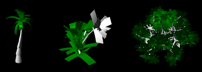
The scene consists of single cottonwood trees, but the underlying algorithm based on Stochastic Lindermayer Systems [Lin68] which can produce a large variety of flora as shown above. The idea is that an n-ary tree is created with geometric annotations consisting of length and radius, and relative position, yaw, and pitch to its parent node. Internal nodes of the tree are rendered as branches or stems, while leaf nodes as groups of leaves, flowers, fruits and so on. Depending on the type of plant one wishes to generate, these parameters take on different values, and the construction of the n-ary tree varies. For a palm tree, a linked list is created, whereas a flower may have several linked lists sharing a common head, and a bush may be a factorial tree with a regular pitch.

Smoke

Fig. 7: Examples of smoke plumes generated using random particles, Metaballs, and Marching Tetrahedra algorithms.

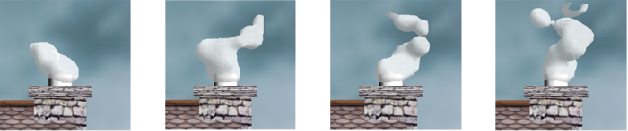
The primary algorithmic challenge of the project was to visualize smoke coming from the chimney of the cabin in the scene. To achieve this, a simple particle system was written in conjunction with [Bli82]’s Metaballs and [PT+90]’s Marching Tetrahedra algorithms. The tetrahedral variant was chosen since it easier to implement from scratch than [LC87]’s original Marching Cubes algorithm. The resulting smoke plumes produced from this chain of algorithms is shown above.

Fig. 8: Visual explanation of the smoke generation process in two dimensions.

Particles possess position and velocity three dimensional components, and are added at a fixed interval to the system in batches with random initial values on the xy-plane and zero velocity terms. A uniform random vector field is created with random x, y components and fixed, positive z component. Euler’s Forward Method is applied to the system to update each particle’s position and velocity. Any particles that escape from the unit bounding cube are removed from the system. This process produces the desired Brownian paths that are typical of smoke particles. To visualize each particle, the Metaballs algorithm is used to create a potential field about each particle. The three dimensional grid is populated in linear time with respect to the number of particles by iterating over a fixed volume about each particle since there is no need to go outside of the fixed volume where the point’s potential field is surely zero.

Fig. 9: Cube segmented into 6 tetrahedra, and the two primary cases of the Marching Tetrahedra algorithm.

The resulting scalar field from this process is passed along to the Marching Tetrahedra algorithm. The algorithm will inspect each volume of the grid in cubic time with respect to the grid edge size. The eight points of the volume are then assigned inside / outside labellings with those volumes completely inside or outside ignored. Those having mixed labellings contain a segment of the surface we wish to render. A single volume is segmented into 6 tetrahedra^[1], with two tetrahedra facing each plane resulting in a common corner shared by all as shown above. Each tetrahedron then has sixteen cases to examine leading to different surfaces. Two of these cases are degenerate; all inside or all outside. The remaining fourteen cases can be reduced to two by symmetry as shown above. To ensure the surface is accurate, the surface vertices are found by linearly interpolating between inside / outside grid points.

Face normals can be computed directly from the resulting surface planes by taking the usual cross product. In order to calculate vertex normals, numerical differentiation is used to derive the gradient of the scalar field at the grid point using backward, central, and forward differences depending on availability. Taking the calculated normals at each grid point, the surface normals at the previously interpolated surface vertices are then the linear interpolation of the corresponding grid point normals. Given more time, I would have liked to put more time into surface tracking and related data structures to reduce the cubic surface generation process down to just those volumes that require a surface to be drawn.

Butterflies

Fig. 10: Example series of movements and completed pursuit curve of predator and prey.

For the final stretch goal, the proposed static options were eschewed in favor of adding in a dynamic element that would help bring the scene to life without being obtrusive. As a result, a kaleidoscope of butterflies that meander through the scene were introduced.

Each butterfly follows a pursuit curve as it chases after an invisible particle following a random walk. Both butterfly and target are assigned positions drawn from a uniform random variable with unit support. At the beginning of a time step, the direction to where the particle will be at the next time step from where the butterfly is at the current time step is calculated, and the butterfly’s position is then incremented in that direction. Once the particle escapes the unit cube, or the butterfly catches the particle, then the particle is assigned a new position, and the game of cat and mouse continues.

Each time step the butterfly’s wings and body are rotated a slight amount by a fixed value, and by the Euler angles defined by its direction to give the correct appearance of flying. To add variety to the butterflies, each takes on one of three different appearances (Monarch, and Blue and White Morpho varieties) based on a fair dice roll. One flaw with the butterflies is that they do not take into account the positions of other objects in the scene and can be often seen flying into the ground, or through the cabin.

Conclusions

This project discussed a large variety of topics related to introductory computer graphics, but did not cover other details that were developed including navigation, camera control, lighting, algorithms for constructing basic primitives, and the underlying design of the C++ program or implementation of the GLSL shaders. While most of the research applied to this project dates back nearly 35 years, the combination of techniques lends to a diverse and interesting virtual environment. Given more time, additional work could be done to expand the scene to include more procedurally generated plants, objects, and animals, as well as additional work done to make the existing elements look more photorealistic.

References

[Bli82] James F. Blinn. A generalization of algebraic surface drawing. ACM Trans. Graph., 1(3):235-256, 1982.

[FFC82] Alain Fournier, Donald S. Fussell, and Loren C. Carpenter. Computer render of stochastic models. Commun. ACM, 25(6):371-384, 1982.

[LC87] William E. Lorensen and Harvey E. Cline. Marching cubes: A high resolution 3d surface construction algorithm. In Proceedings of the 14th Annual Conference on Computer Graphics and Interactive Techniques, SIGGRAPH 1987, pages 163-169, 1987.

[Lin68] Astrid Lindenmayer. Mathematical models for cellular interactions in development i. filaments with one-side inputs. Journal of theoretical biology, 18(3):280-299, 1968.

[PT+90] Bradley Payne, Arthur W Toga, et al. Surface mapping brain function on 3d models. Computer Graphics and Applications, IEEE, 10(5):33-41, 1990.